Form Factors & Structure factors¶

This is list of available form factor and structure factors in Irena package.

Form & Structure factors parameters¶

´User uses user provided functions.

There are two user provided functions necessary -: F(q,R,par1,par2,par3,par4,par5)

and V(R,par1,par2,par3,par4,par5) the names for these need to be provided in strings...

the input is q and R in angstroms

Important comment for Core-shell and Core shell cylinder (and Unified tube). The volume definition for Core-shell objects is matter of discussion. Heated at times and I suspect that the appropriate answer depends on the case when and how the FF is used. Therefore from version 2.26 Irena macros include option which needs to be set - both Core shell and Core shell cylinder will share common parameter (this parameter is global for all cases of calls to core shell form factors or their volumes) of volume definition. The options are: whole particle, core, and shell

Note: Unified tube is using as volume the volume of shell. It is how it is defined at this time and it is meant for cases like Carbon nanotubes, when this is appropriate. To match with core shell cylinder us “shell” as volume

Form Factor description¶

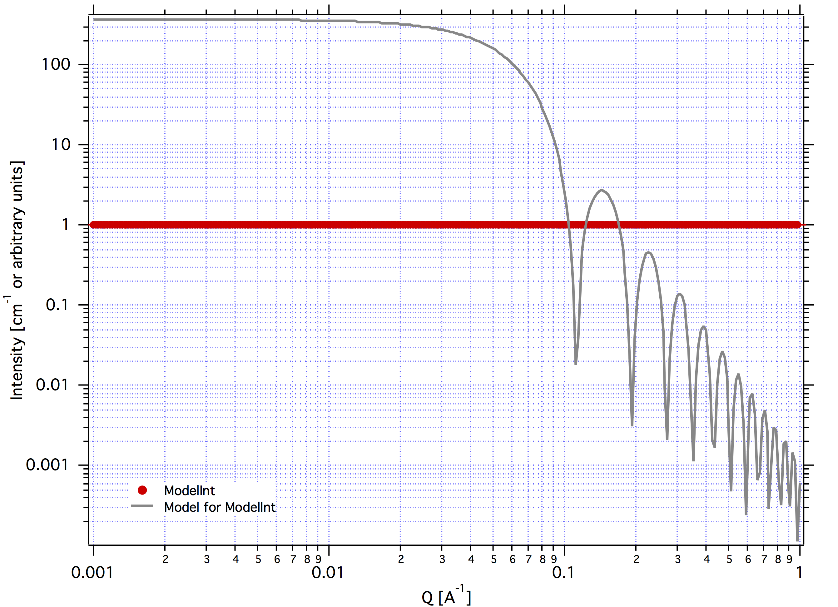
Spheroid¶

uses sphere form factor for aspect ratio between 0.99 and 1.01:

F^2 = 3/(QR^3))*(sin(QR)-(QR*cos(QR))

volume : V=((4/3)*pi*radius^3)

This calculation approximates integral over R as rectangle (compare with Integrated spheroid).

graph for R = 50A

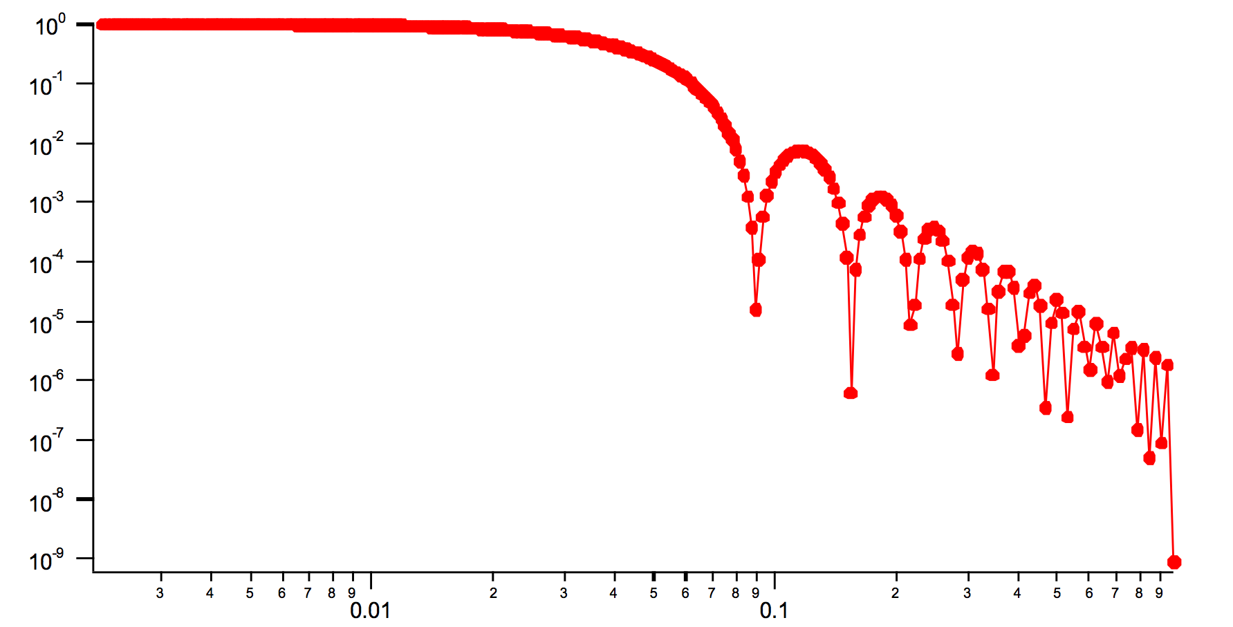
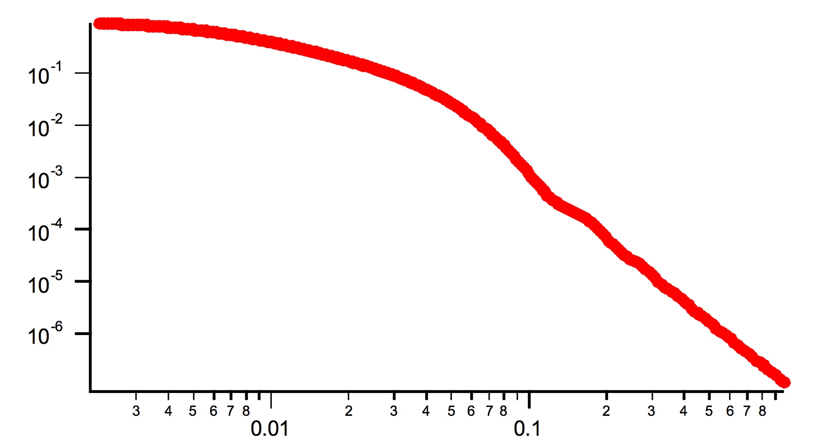
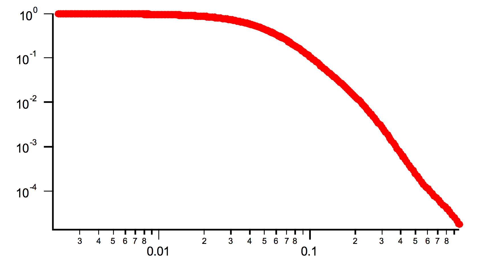
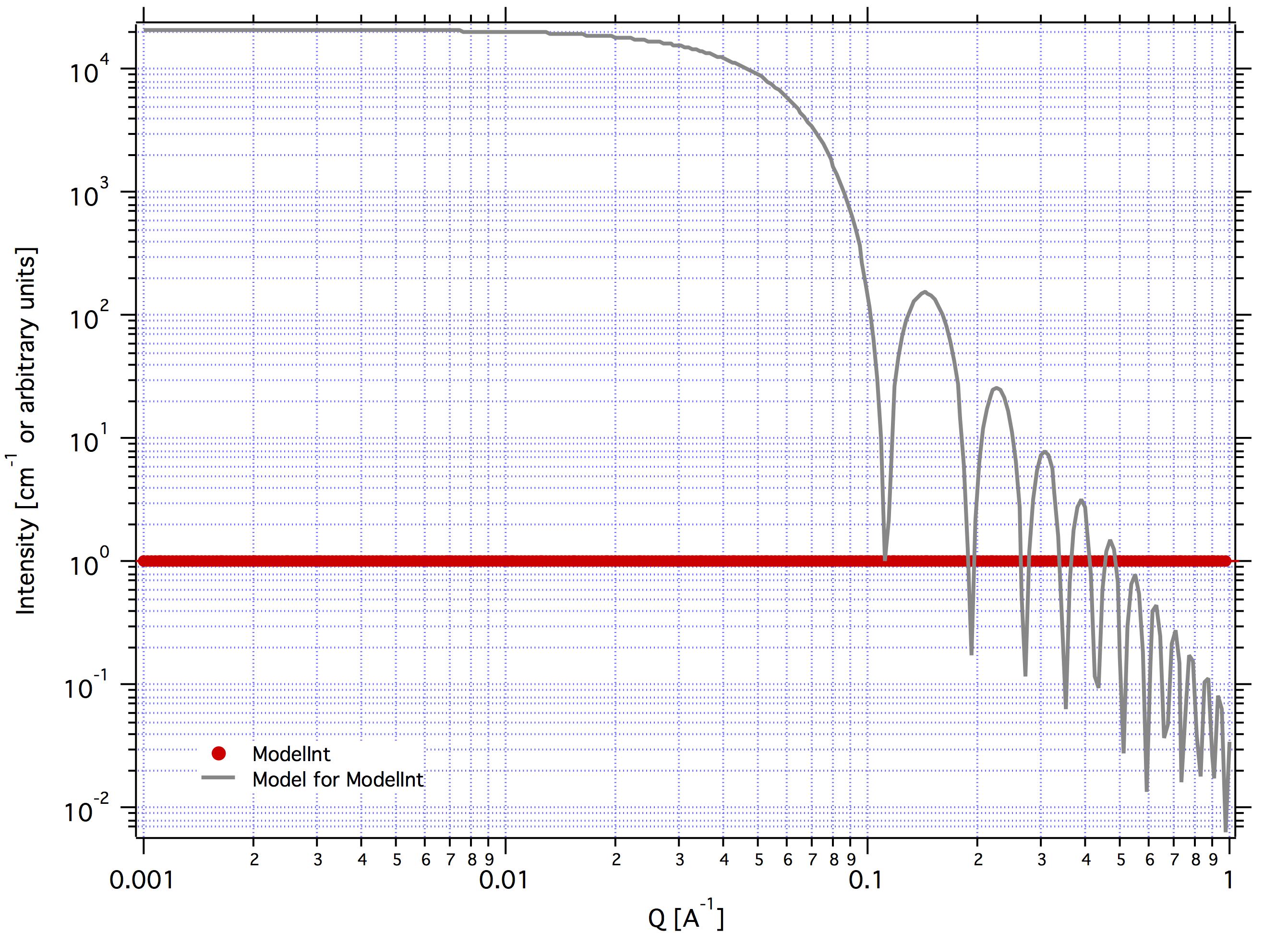
For aspect rations smaller than 0.99 and larger than 1.01 uses standard form factor for spheroid:

F = Integral of (3/(QR^3))*(sin(QR)-(QR*cos(QR)))

where QR=Qvalue*radius*sqrt(1+(((AR^2)-1)*CosTh^2))

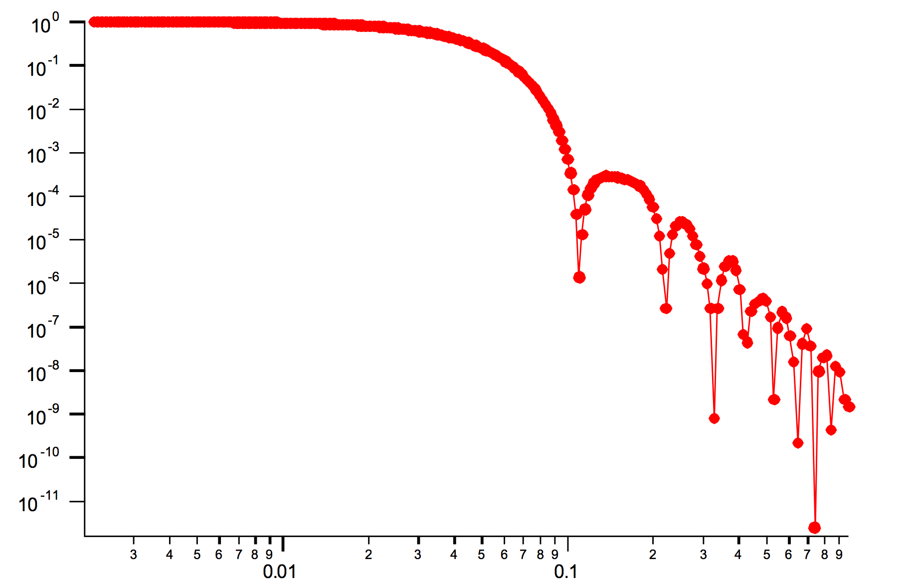
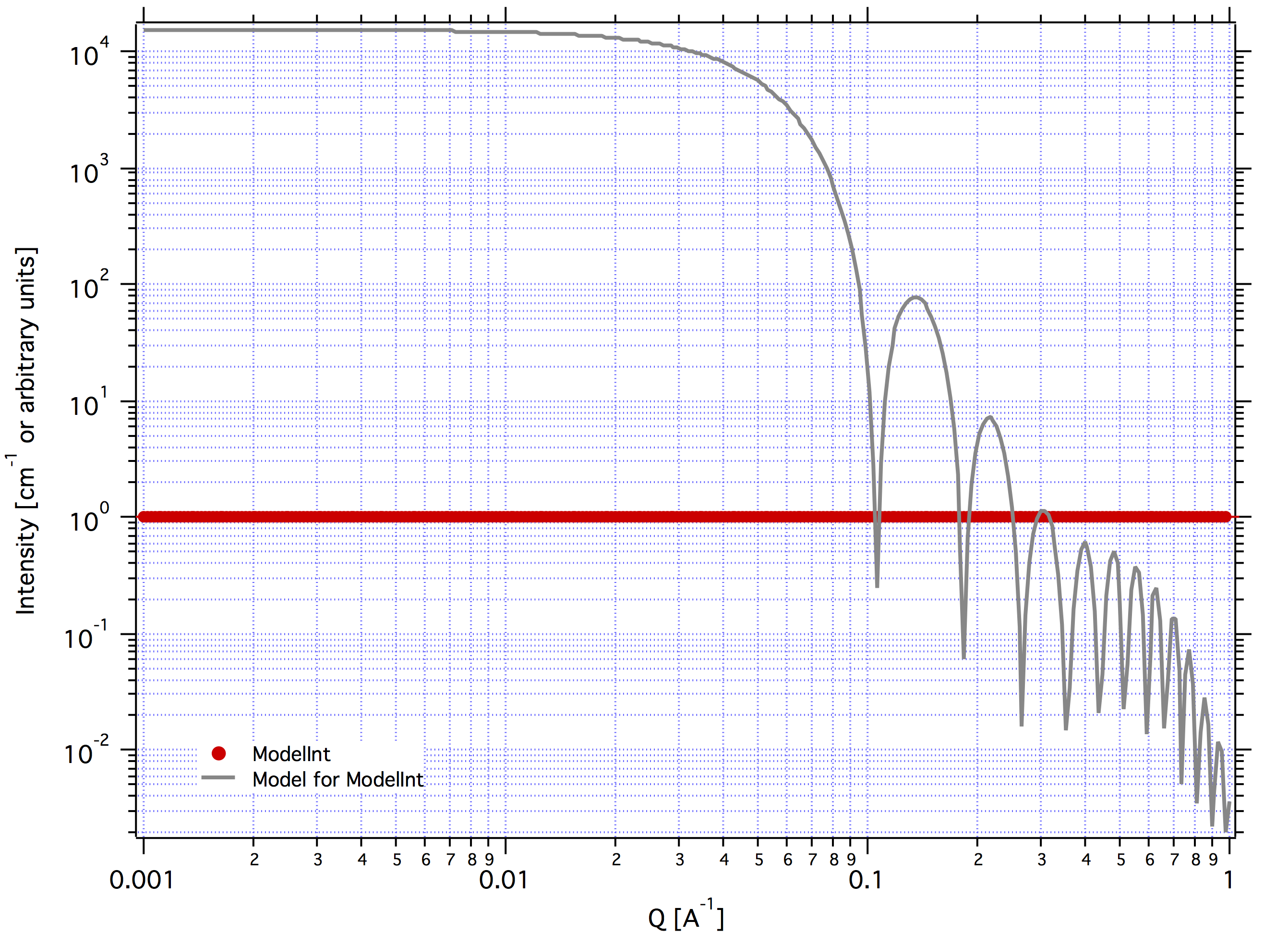
over of CosTh = 0 to 1. This is numerically calculated using 50 points (step in CosTh = 0.02). Following graphs are examples:

AR = 10

AR=0.1

Since Irena version 2.54 Spheroid with aspect ratio !=1 will use NIST xop to speed up its calculations.

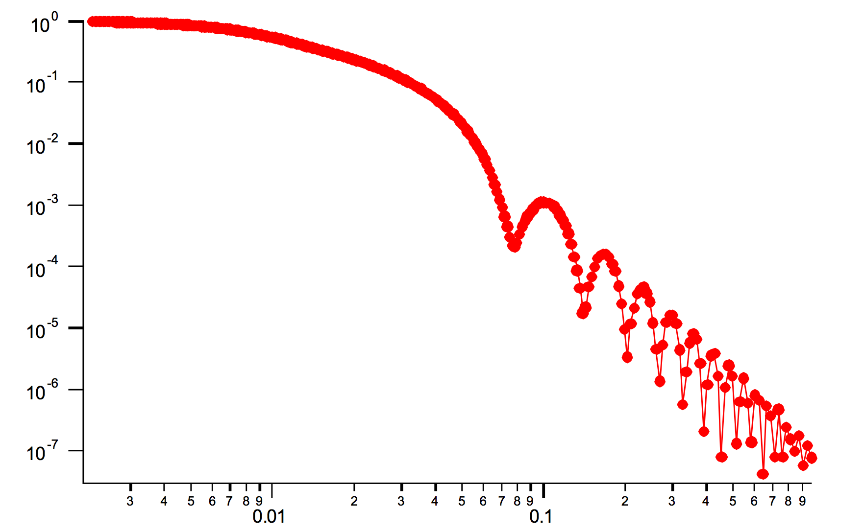
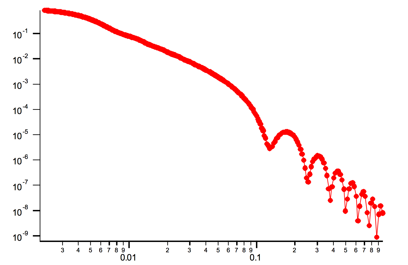
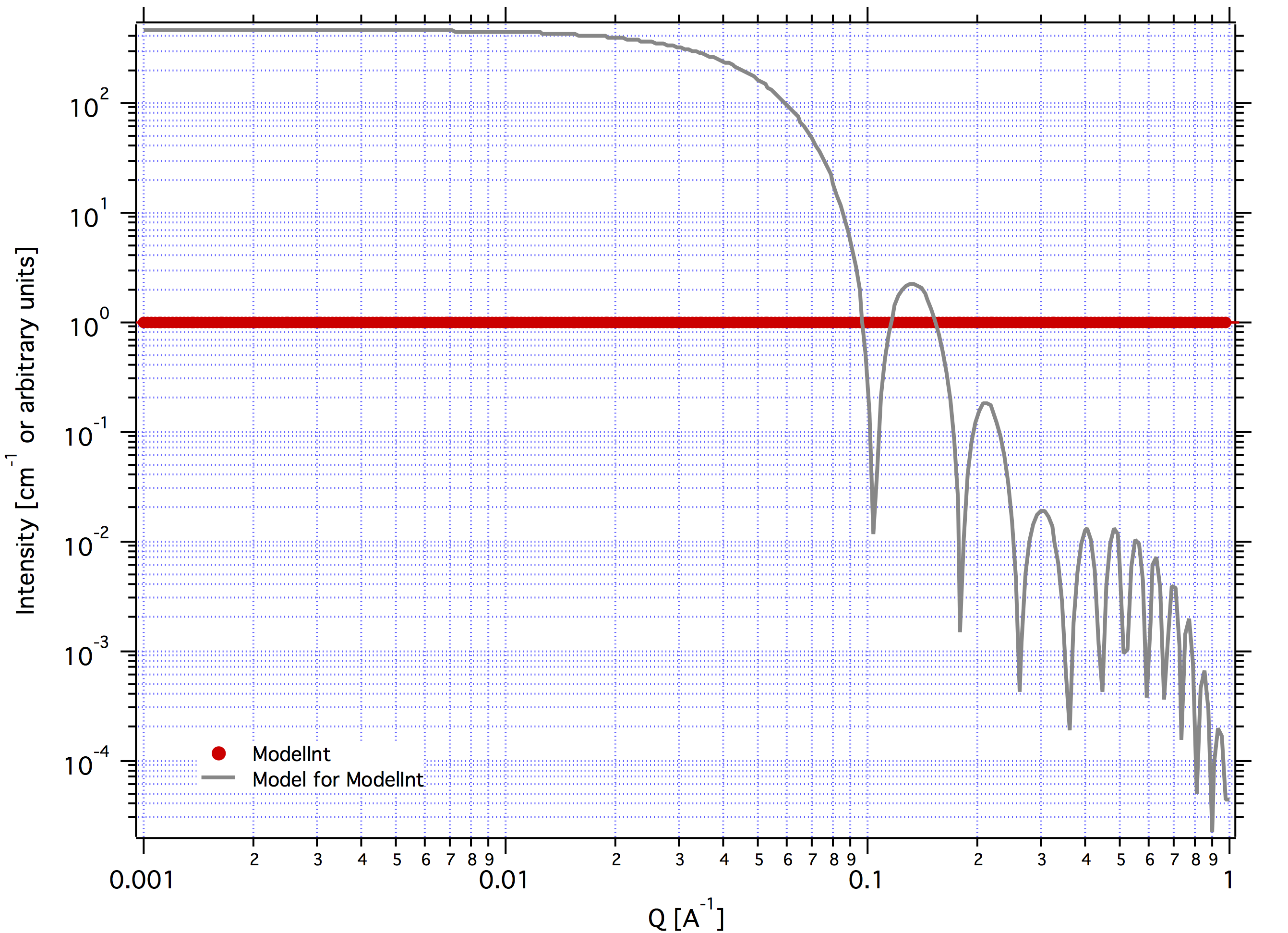
Integrated_Spheroid¶

same code as in the spheroid, but in this case the code integrates over the width of the R bin. Note, the bin star and end points are calcualted linearly (even for log-binned data) as half way distance:

Rstart = (Rn + Rn-1)/2 Rend = (Rn + Rn+1)/2 Uses adaptive steps to integrate essel function oscillations of the form factor over the width of the bin in R - note, the averaging is done including the volume of particles involved. This code is quite convoluted and time consuming. Its only reasonable use is for cases with wide bins in radius (R), when this removes some of the bessel function oscillations.

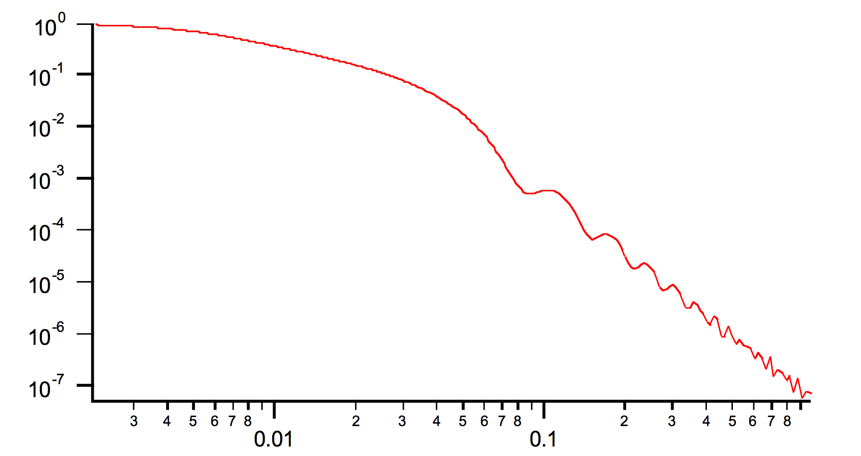
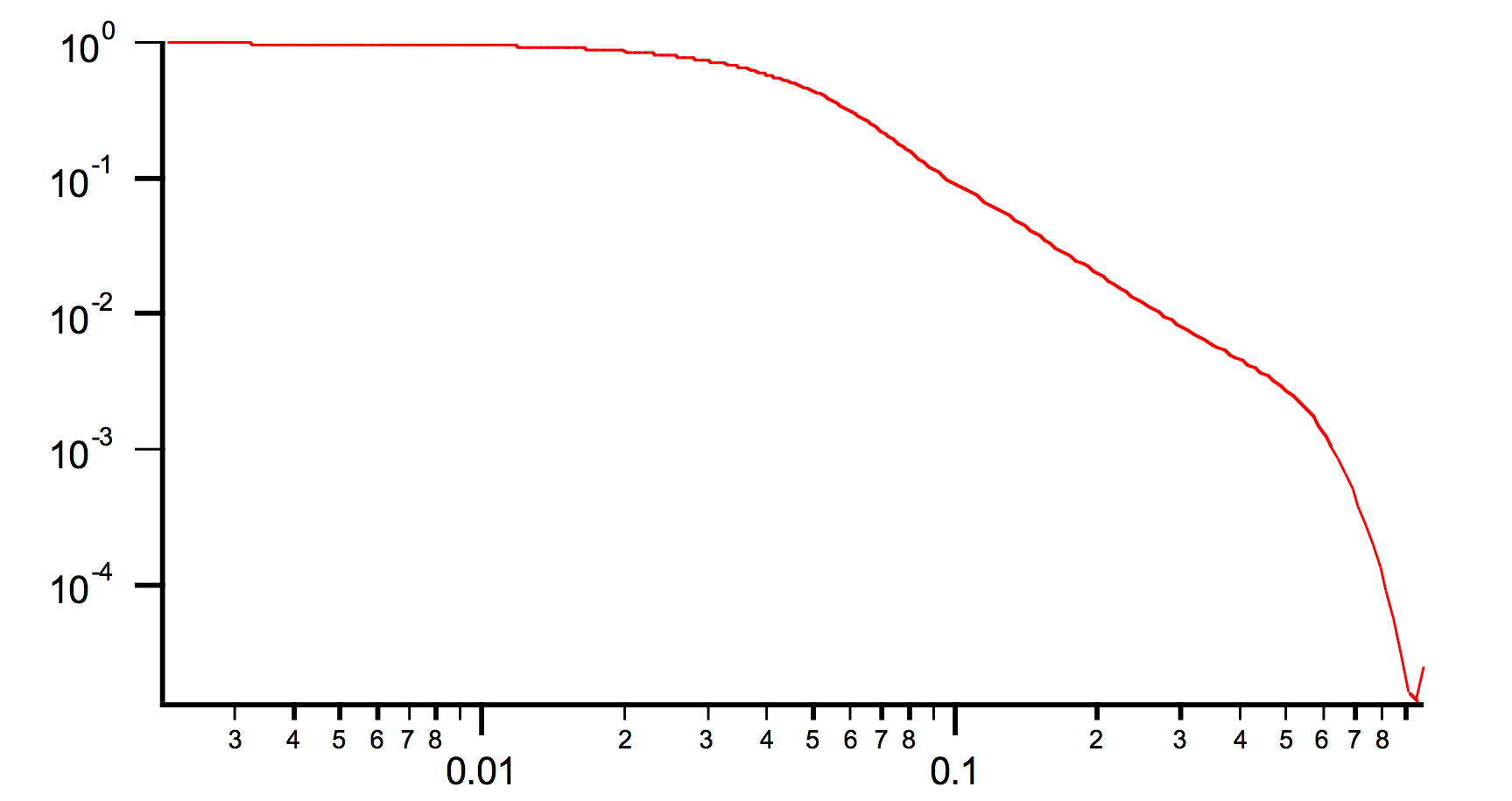
Examples with R width 40A, average size 50A (that means R varies from 30 to 70A). Note that the bessel function oscillations are somewho smooth out. With wider bins in R these oscillations may disappear all together.

AR = 1 (sphere)

AR=10 (Spheroid)

AR=0.1 (spheroid)

Cylinder and CylinderAR¶

The code uses the following code to calculate form factor for cylinder. Note, that also this code is doing the same integration as integrated spheroid above (see 2).

Form factor = integral over (Ft) for Alpha = 0 to pi/2, Ft is below: LargeBes=sin(0.5*Qvalue*length*Cos(Alpha)) / LargeBesArg SmallBessDivided=BessJ(1, Qvalue*radius*Sin(Alpha))/Qvalue*radius*Sin(Alpha) Ft = LargeBes*SmallBessDivided

Examples Cylinder with length 500A and radius 50A.

Disk (cylinder) with radius 500A and length 50A.

Since Irena version 2.54 Cylinders will use NIST xop to speed up its calculations.

Unified_Sphere¶

This is formula from Unified fit model by Greg Beaucage (see Unified tool and documentation for it). The parameters are calculated from the code in the manual for each different shape. Specific formulas for these shapes were provided by Dale Schaefer...

This is the code:: G1=1 P1=4 Rg1=sqrt(3/5)*radius B1=1.62*G1/Rg1^4 QstarVector=qvalue/(erf(qvalue*Rg1/sqrt(6)))^3 F^2 = G1*exp(-qvalue^2*Rg1^2/3)+(B1/QstarVector^P1)

Example for R=50A compared with the spheroid with aspect ratio =1

Unified_Rod¶

Unified_RodAR¶

This is the code:: G2 =1 Rg2=sqrt(Radius^2/2+Length^2/12) B2=G2*pi/length P2=1 Rg1=sqrt(3)*Radius/2 RgCO2=Rg1 G1=2*G2*Radius/(3*Length) B1=4*G2*(Length+Radius)/(Radius^3*Length^2) P1=4 QstarVector=qvalue/(erf(qvalue*Rg2/sqrt(6)))^3 A=G2*exp(-qvalue^2*Rg2^2/3)+(B2/QstarVector^P2) * exp(-RGCO2^2 * qvalue^2/3) QstarVector=qvalue/(erf(qvalue*Rg1/sqrt(6)))^3 F^2 = A + G1*exp(-qvalue^2*Rg1^2/3)+(B1/QstarVector^P1)

Example for R=50A and length 500A compared with the cylinder

Unified_Disk¶

This is the code:: G2=1 Rg2=sqrt(Radius^2/2+thickness^2/12) B2=G2*2/(radius^2)//dws guess P2=2 Rg1=sqrt(3)*thickness/2// Kratky and glatter = Thickness/2 RgCO2=1.1*Rg1 G1=2*G2*thickness^2/(3*radius^2) B1=4*G2*(thickness+Radius)/(Radius^3*thickness^2)//same as rod P1=4 QstarVector=Q/(erf(Q*Rg2/sqrt(6)))^3 A=G2*exp(-Q^2*Rg2^2/3)+(B2/QstarVector^P2) * exp(-RGCO2^2 * Q^2/3) QstarVector=Q/(erf(Q*Rg1/sqrt(6)))^3 F^2 = A + G1*exp(-Q^2*Rg1^2/3)+(B1/QstarVector^P1)

Example for R=250A and thickness 10A compared with the cylinder

CoreShell¶

One thing to remeber: the total radius of this particle is core radius + shell thickness... If you use diameter as dimension of the particle (new in Irena version 2.53), the total diameter of the particle is diameter+2*shell thickness. Note, this form factor calculation also includes integration over the width of bin in radii (same as integrated spheroid and cylinder).

Note: Input form factor parameter for core/shell/solvant is rho in [1010 cm-2] - this is very important to keep in mind.

Note, that there is volume definition choice you need to do: Whole particle, core, or shell, as appropriate for given problem. This volume definition is used for all volume calculations for this particle. It is global parameter for all core shell cylinder or core shell calls in the WHOLE EXPERIMENTÅc.

Code (heavily simplified!):

RhoDelta = CoreRho - ShellRho //core Result1=(3/(Q*R)^3)*(sin(Q*R)-(Q*R*cos(Q*R))) * RhoDelta * (4/3 * pi * R^3)

//Now add the shell (skin) , thickness Rshell r = R+Rshell RhoDelta = ShellRho - SolventRho Result2 = (3/(Q*r)^3)*(sin(Q*r)-(Q*r*cos(Q*r))) * RhoDelta * (4/3 * pi * r^3)

//summ them together and normalize by the total particle volume F^2 =( result1 + result2 )^2 / Volume

Volume definition depends on the setting of above discussed global parameter and is either: Whole particle volume = 4/3 * pi * (R+r)^3 Core volume = 4/3 * pi * R^3 Shell volume = 4/3 * pi * (R+r)^3 - 4/3 * pi * R^3

Make sure your choice is appropriate

Note, that to my surprise these calculations (copied from NIST Form factors) do not normalize correctly to 1 at low q. The reason is that the weighting is done by volume and contrast. I’ll need to look into this again and in detail...

Example, Radius 50A, skin thickness 10A, contrast ratio 0.6

CoreShellPrecipitate¶

This is unique form factor, which - even for dilute sytem - results in “diffraction peak” type scattering. It is a very special case, when coreshell particle is formed from matrix and as it is formed, the core chemistry/rho deviates from matrix chemistry/rho. If the diffusion in the matrix is not fast enough, the chemistry around the particle changes, which results in rho changing in the other direction. Therefore one can end with coreshell particle which has higher-then-solvent rho core surounded by lower-then-solvent rho shell (or the other way). With average rho same as matrix. In such case at low-qs the particle “disappers” since we are probing material on larger length scales, and on average at those length scales the rho is the same. Fro example of this type of precipitation see:

Imhoff, S.D., et al., Kinetic transition in the growth of Al nanocrystals in Al-Sm alloys. Journal of Applied Physics, 2012. 111(6): p. 063525-9.

Remember, that by basic nature of this logic, the rho of the core/shell needs to be one larger and the other smaller than solvent rho. Also, they probably need to be pretty close together. If this is not correct, the code would create negative shell thicknesses and abort. Do not do it, it is not very physical...

The particle volume is always volume of the core. I think no other logic makes too much sense.

Code uses regular coreshell form factor (see above). For each size the shell thickness is calculated so the average rho of the particle matches the rho of the solvent. First we calculate: ShellVolume = CoreVolume*(SolventRho - CoreRho) / (ShellRho - SolventRho) Then we calculate the shell thickness for known ShellVolume and known core radius. Core volume = 4/3 * pi * R^3

Example, Radius 50A, Core Rho 110, Shell Rho 85, Solvent Rho 90; note, this internally resolves to shell thickness of 35.5A.

../_images/FormFactor_CoreShellPrecip.png

CoreShell Cylinder¶

Note, this form factor calculation also includes integration over the width of bin in radii (same as integrated spheroid and cylinder).

This code has been developed some time ago and I am not sure about it’s function...

Code which is being used is direct copy of NIST Core shell cylinder.

Volume definition depends on the setting of above discussed global parameter and is either: Whole particle volume = pi * (R+r)^2 * (L+2*r) Core volume = pi * R^2 * L Shell volume = pi * (R+r)^2 * (L+2*r) - pi * R^2 * L

Fractal Aggregate¶

This form factor was requested by Dale Schaefer and I cannot very well guarantee its functionality....

code:

f = IR1T_CalcSphereFormFactor(Qw[p],(2*Param1)) //calculates the F(Q,r) part fo formula //this is same as for sphere of diameter = 2*Param1 //(= radius of primary particle, which is hard sphere) //fractal part is next F^2 =f^2 * IR1T_CalculateFractAggSQPoints(Qw[p],currentR,Param1, Param2)

where IR1T_CalculateFractAggSQPoints(Qvalue,R,r0, D) is

QR=Qvalue*R part1=1 part2=(qR*r0/R)^-D part3=D*(exp(gammln(D-1))) part5= (1+(qR)^-2)^((D-1)/2) part4=abs(sin((D-1)*atan(qR)))

return (part1+part2*part3*part4/part5)

Note, that parameters are : Param1 - radius of primary particle param2 - fractal dimension of the fractal particles

Example for R=100A, radius of primary particle 10 A and fractal dimension 2.5.

Comment: Note, that this is not scaled correctly at all... I have no idea why - apparently this formula is either wrongly coded or plainly does not behave right.

CoreShellShell¶

This form factor has been provided by Fan Zhang, many thanks to him. Description of the model:

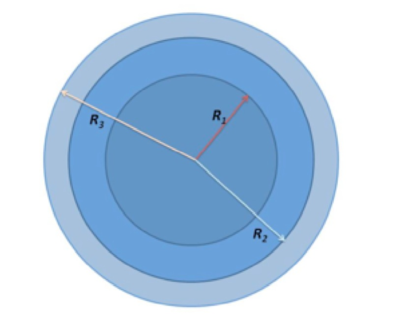
Scattering Length Density Rho:

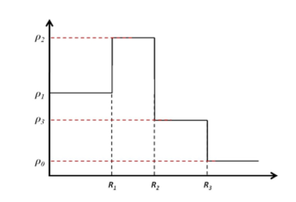
../_images/FormFactor_CoreShellShell2.png

List of Model Parameters: R1 : core radius R2 : outer radius of the first shell R3 : outer radius of the second shell : scattering length density of the matrix

: scattering length density of the core

: scattering length density of the first shell: : scattering length density of the second shell

First-order Bessel function of the first kind is defined as

Volume is defined as

add formula here

Form factor of the core-shell-shell structure is:

add formula here...

Volume definition depends on the setting of global parameter described in Core-shell form factor and is either: Whole particle volume = 4/3 * pi * (R+r)^3 Core volume = 4/3 * pi * R^3 Shell volume = 4/3 * pi * (R+r)^3 - 4/3 * pi * R^3 Where shell thickness “r” is sum of the two shell thicknesses (R3-R1). Make sure your choice is appropriate

SphereWHSLocMonoSq¶

This is form factor combined with structure factor – Based on Jan Skov Pedersen J. Appl. Cryst paper : J. Appl. Cryst. (1994) 27, 595-608. The model is locally mono dispersed system, therefore locally one can use spheres Form factor combined with structure factor. For each bin here the code calculates F(Q,R)^2 * S(Q,D,phi), where D ~ R via input parameter. Phi is simply fraction of Percus Yevic structure factor.

The result is different than multiplying dilute system by Structure factor – that assumes that the distance for Structure factor is the same for all sizes. In this case the ratio of distance to size of particle is the same. We assume here that the phi is the same for all sizes.

Suffise to say, that using this form factor with another structure factor is meaningless and garbage will be produced.

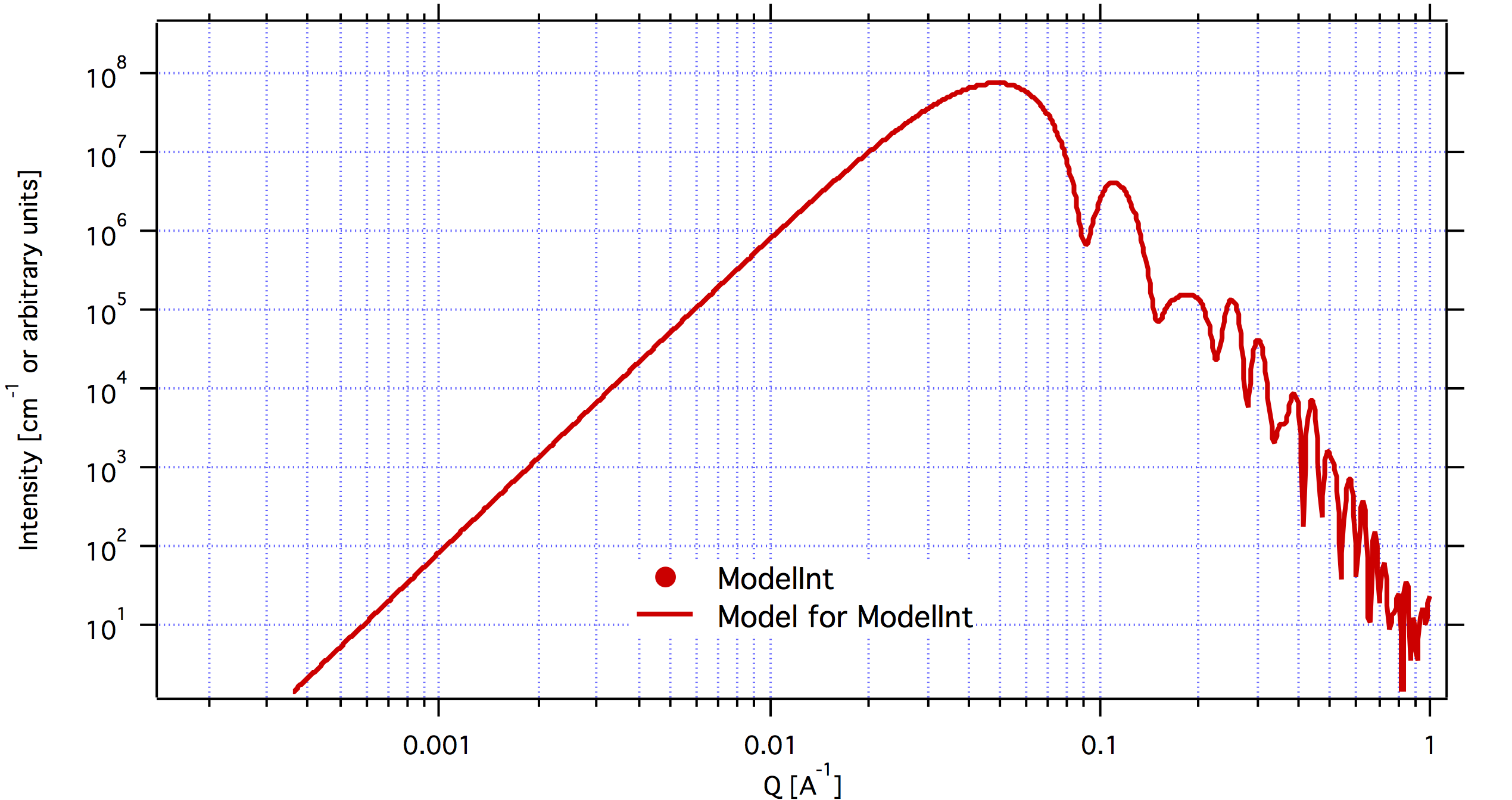
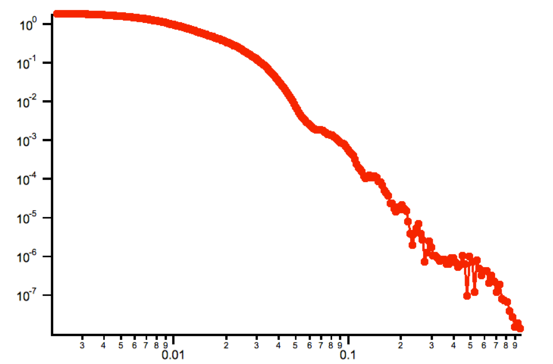
Janus CoreShell Micelle¶

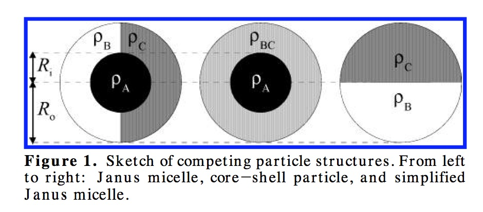
This is form factor based on manuscript: T. Futterer, G. A. Vliegenthart, and P. R. Lang, “Particle Scattering Factor of janus Micelles”, Macromolecules 2004, 37, 8407-8413. The Form factor follows formula 3 of this manuscript

which describes scattering from the particle on the left of the Figure 1 from their manuscript (below).

Example of results:

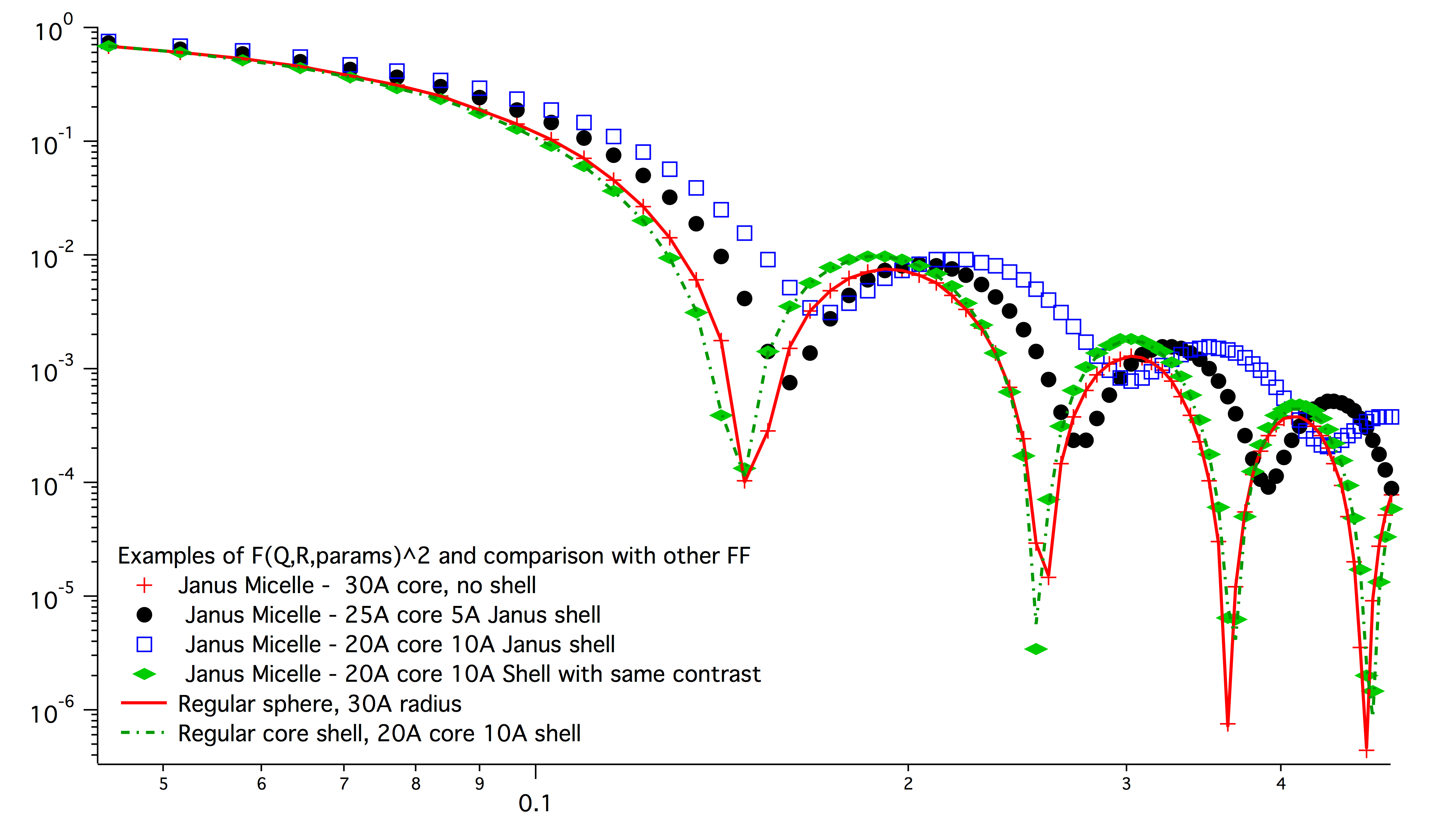
Note: the results in the above graph are scaled to F^2(Q=0) = 1. Since the formula inclused scattering length densities, normalization by the volume does not result in F^2(Q=0) = 1. This may result in unexpected problems with absolute calibration.

This FF is implemented twice...

“Janus CoreShell Micelle 1” ... particle size is total size of the particle (R0 in the figure in description), parameters:: Shell_Thickness=ParticlePar1 //shell thickness A CoreRho=ParticlePar2 // rho for core material Shell1Rho=ParticlePar3 // rho for shell 1 material Shell2Rho=particlePar4 // rho for shell 2 material SolventRho=ParticlePar5 // rho for solvent material
“Janus CoreShell Micelle 2” ... particle size here is shell thickness!!! This may be _very_ confusing!!!!, parameters:: Core_Size=ParticlePar1 // Core radius A CoreRho=ParticlePar2 // rho for core material Shell1Rho=ParticlePar3 // rho for shell 1 material Shell2Rho=particlePar4 // rho for shell 2 material SolventRho=ParticlePar5 // rho for solvent material
“Janus CoreShell Micelle 3” ... particle size is radius of the core (Ri in the figure in description), parameters:: Shell_Thickness=ParticlePar1 //shell thickness A CoreRho=ParticlePar2 // rho for core material Shell1Rho=ParticlePar3 // rho for shell 1 material Shell2Rho=particlePar4 // rho for shell 2 material SolventRho=ParticlePar5 // rho for solvent material

The reason for the two implementations is, that in usual implementation the shell thickness is fixed while the particle size has size distribution - but this is possible ONlY if core has distribution of sizes. This may be incorrect, as someone can have monodispersed cores, but distribution of shell thicknesses.

Note, that the “Janus CoreShell Micelle 2 and 3” will not work with some of the tools in Irena as all assume size represents total size (core+shell). Be warned, results will be difficult to present meaningfully! You are on your own...

Model comparison: Core (Au): 131.5 10^10cm^-1 Shell 1 (Al2O3) 34.95 10^10 Shell 2 (ZrO2) 46.27 10^10 Solvant (H2O) 9.42 10^10 volume = 0.05

Janus CoreShell Micelle 1: Mean radius 40A, width 0.3A (Gauss), Shell thickness 10A,

Janus CoreShell Micelle 2: Core radius 30A, Mean radius 40A, width 0.3A (Gauss) :

Janus CoreShell Micelle 1: Pseudo sphere (shell thickness = 0), Radius = 40 A,

Real sphere, contrast 14903.5 (Au-water):

Note the suspicious difference in calibrations. See note above about my suspicion on the problem here...

Real core shell system (pick shell contrast 34.95). Use “Whole particle” as volume.

Janus CoreShell Micelle 1, fake the core shell with same contrast (34.95) for both shells. Recall that the total size of the CoreShell in Irena is radius of core (“Radius”)+ shell thickness; while for Janus CoreShell Micelle 1 it is just Radius (see figure).

The difference in absolute intensity here is surely related to different assumptions on volume of particle.

RectParallelepiped¶

This is form factor or rectangular Parallelpiped, cuboid shape with side A x B x C and all angle 90 degrees. This form factor is ONLY available if NIST form factor xop is installed on the computer. If you install NIST SANS package http://www.ncnr.nist.gov/programs/sans/data/red_anal.html it installs xop which provides fast calculations of the various form factors. Since version 2.53 Irena will take advantage of some of these form factors. In the case of rectangular Parallelpiped see NIST form factor description. It seems they had to go to original manuscript and recreate the form factor from the German original, Mittelbach and Porod, Acta Phys. Austriaca 14 (1961) 185-211, equations (1), (13), and (14) (in German!). Most publications citing this form factor seem to be wrong (I think there is error in Pedersen 1997 manuscript I was working with, Steven cites other manuscripts which seem to have bugs in tehm).

If you use this form factor, cite Steven Kline manuscript for NIST package: “Reduction and Analysis of SANS and USANS Data using Igor Pro”, Kline, S. R. J Appl. Cryst. 39(6), 895 (2006).

Here is example of Form factor

Cuboid, 60A sides:

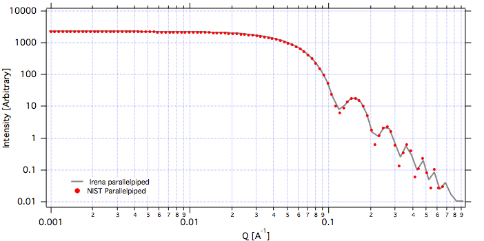
Hereis Parallelepiped with sides 60A, 120A, 180A:

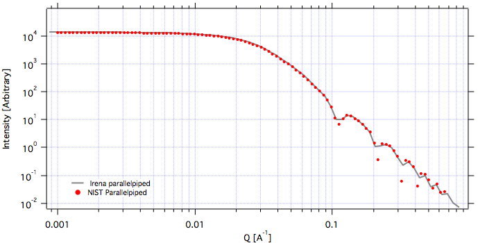
Note, Irena assumed some size distribution (narrow, but some) while NIST package, assumes monodispersed particle. Therefore the differences in oscillations.

User¶

To use “User” form factor you will need to supply two functions: 1. Form factor itself 2. Volume of particle function Both have to be supplied. Use of form factors which would include volume scaling within is possible, but MUCH more challenging due to other parts of code. If you really insist on doing so, contact me and I will create rules and explanation.

Both functions must work with radius in Angstroems and Q in inverse Angstroems. Both have to declare following parameters, in following order:

Form factor: Q, radius, par1,par2,par3,par4,par5 Volume : radius, par1,par2,par3,par4,par5

These function are not required to use these 5 user parameters, but they have to declare them.

Examples for sphere: Function IR1T_ExampleSphereFFPoints(Q,radius, par1,par2,par3,par4,par5) //Sphere Form factor

variable Q, radius, par1,par2,par3,par4,par5 variable QR=Q*radius return (3/(QR*QR*QR))*(sin(QR)-(QR*cos(QR)))

end

Function IR1T_ExampleSphereVolume(radius, par1,par2,par3,par4,par5) //returns the sphere volume

variable radius, par1,par2,par3,par4,par5

return ((4/3)*pi*radius*radius*radius)

end

Testing and using Form factors in users own code¶

To verify that the form factor works for you and to use the form factor if your own functions use following process and functions:

Generate Q wave with Qs for which the data are to be calculated
Generate intensity wave (will be redimesnioned as necessary, so the only thing is, it should be double precision).
Generate distributipon of radii wave - if you want to use single R, create wave with single point
decide what you want to calculate:

F^2 powerFct=0 V*F^2 powerFct=1 V^2 * F^2 powerFct=2

5. Run following command: IR1T_GenerateGMatrix(R_FF,Q_wave,R_dist,powerFct,”form factor name”,param1,param2,param3,param4,param5, “”, “”)

This function will return R_intensity, which is generally matrix with dimensions numpoints(Q_vector) x numpoints(R_dist), if R_dist has 1 point only, returned is wave (vector) as expected and reasonable... The param1 - param5 are form factor parameters, as desribed in chapter 1, the “” at the end are for user form factor functions (there go the strings with names of user form factor and volume function). “form factor name” is name from list in chapter 1.

Create log-log plot of the data if R_dist has single point. If R_dist has more point, well, you have to pull out the right column of data you need to plot.

Note, that if the IR1T_GenerateGMatrix function returns wave of NaN values if unknown name of form factor is passed in.

Example of code:

make/N=100 Q_wave Q_wave=0.001+p/100

//will create 100 points wave with values 0.001 to 1) values

Make/O/D R_FF: //makes some place for form factor

make R_dist R_dist=50 //or //make/N=3 R_dist //R_dist={10,50,100}

//creates R distribution and sets values

IR1T_GenerateGMatrix(R_FF,Q_wave,R_dist,powerFct,”form factor name”,param1,param2,param3,param4,param5, “”, “”): //Note, above lines belong on one line together! // replace powerFct with 0, 1,or 2!

// replace “form factor name” with name of form factor you want to use Display R_FF vs Q_wave ModifyGraph log=1

//creates log-log graph of

Structure factors description¶

This is list of library of structure factors. These structure factors enable to deal with limited S(Q) effects in Irena package. The functionality is provided by library, which can be called by any other user code. The library provides also GUI for setting the user parameters. In principle, further structure factors can be added if they have less than 5 parameters.

Interferences¶

This is original structure factor in Irena package. It has been provided as part of Unified fit model by Gregg Beaucage and is listed in his publication: Beaucage, G. (1995). Chapter 9 in ÅgHybrid Organic-Inorganic CompositesÅh, ACS symposium Series 585, edited by J. E. Mark, C. Y-C. Lee, and P. A. Bianconi, 207th National Meeting of the American Chemical Society, San Diego, CA, March 13-17, 1994. American Chemical Society, Washington, DC 1995. Pg. 97 – 111.

Note, that this model is, for most practical purposes, close to Hard spheres model with different definition of the parameters k (ÅgpackÅh) and ƒÄ (ÅgETAÅh). Modeling II extends the capabilities by including three more structure factors using code available from NIST Igor package (ref). Included are now: Hard spheres, Square Well, and Sticky Hard Spheres, which can be used in addition to interferences model above and no structure factor (dilute limit).

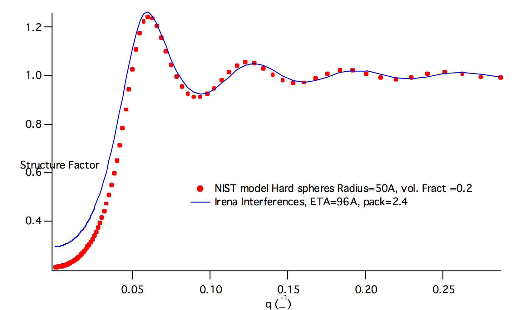
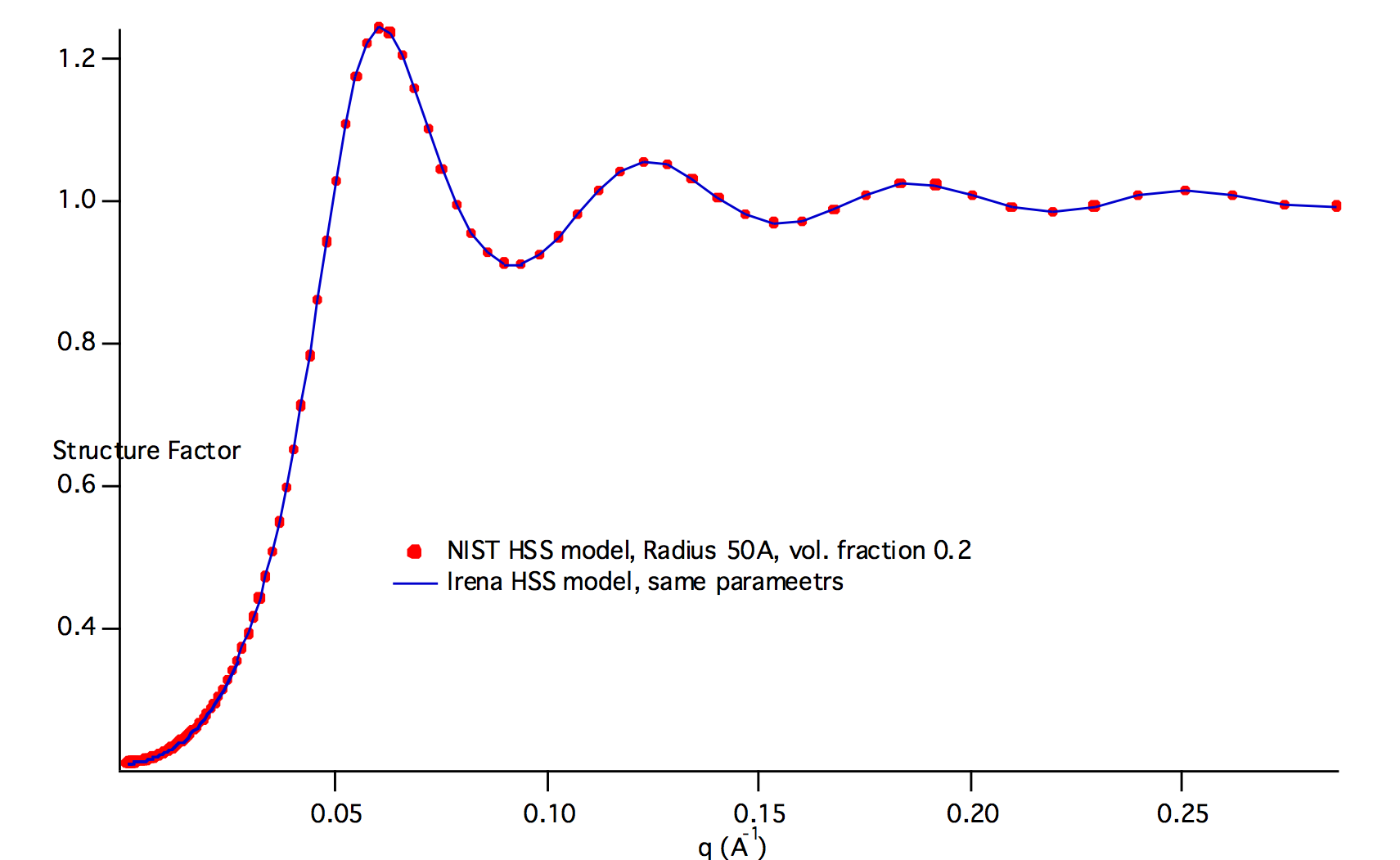
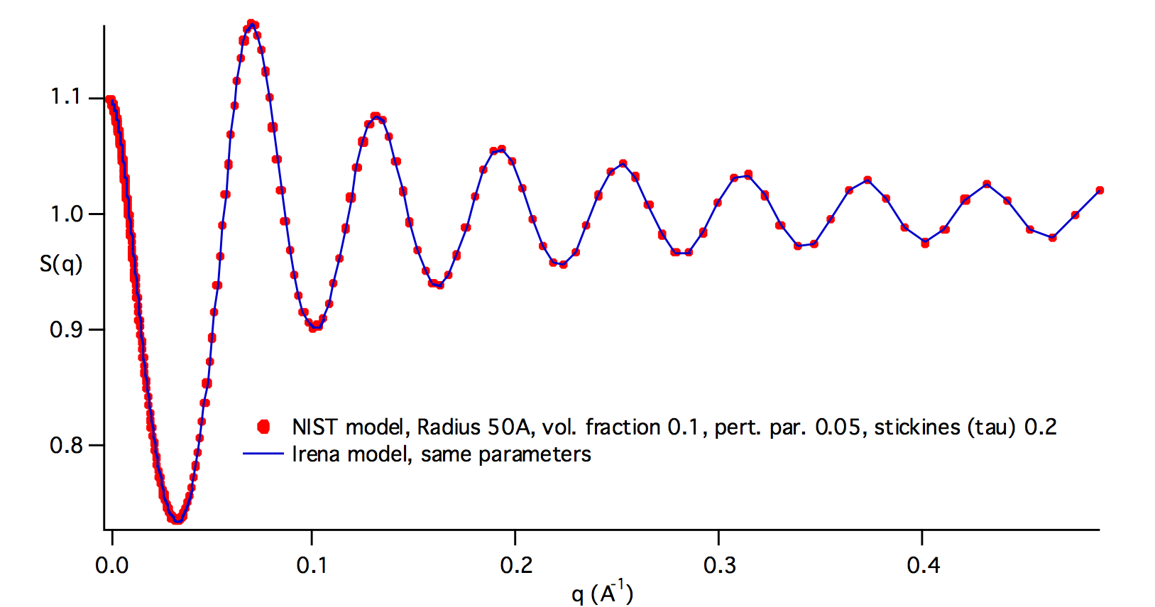
../_images/StructureFactor_Interferences.png

HardSpheres¶

The code for this structure factor has been copied from NIST SAS macros (Kline, S. R. (2006). J Appl Crystallogr 39, 895-900). Please, give them credit when using this structure factor. (http://www.ncnr.nist.gov/programs/sans/data/data_anal.html)Åc

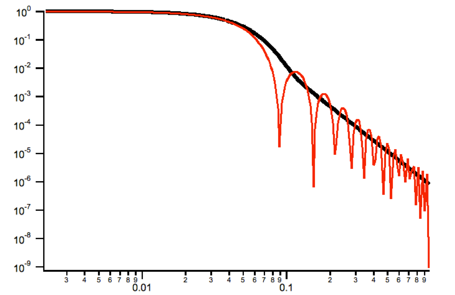
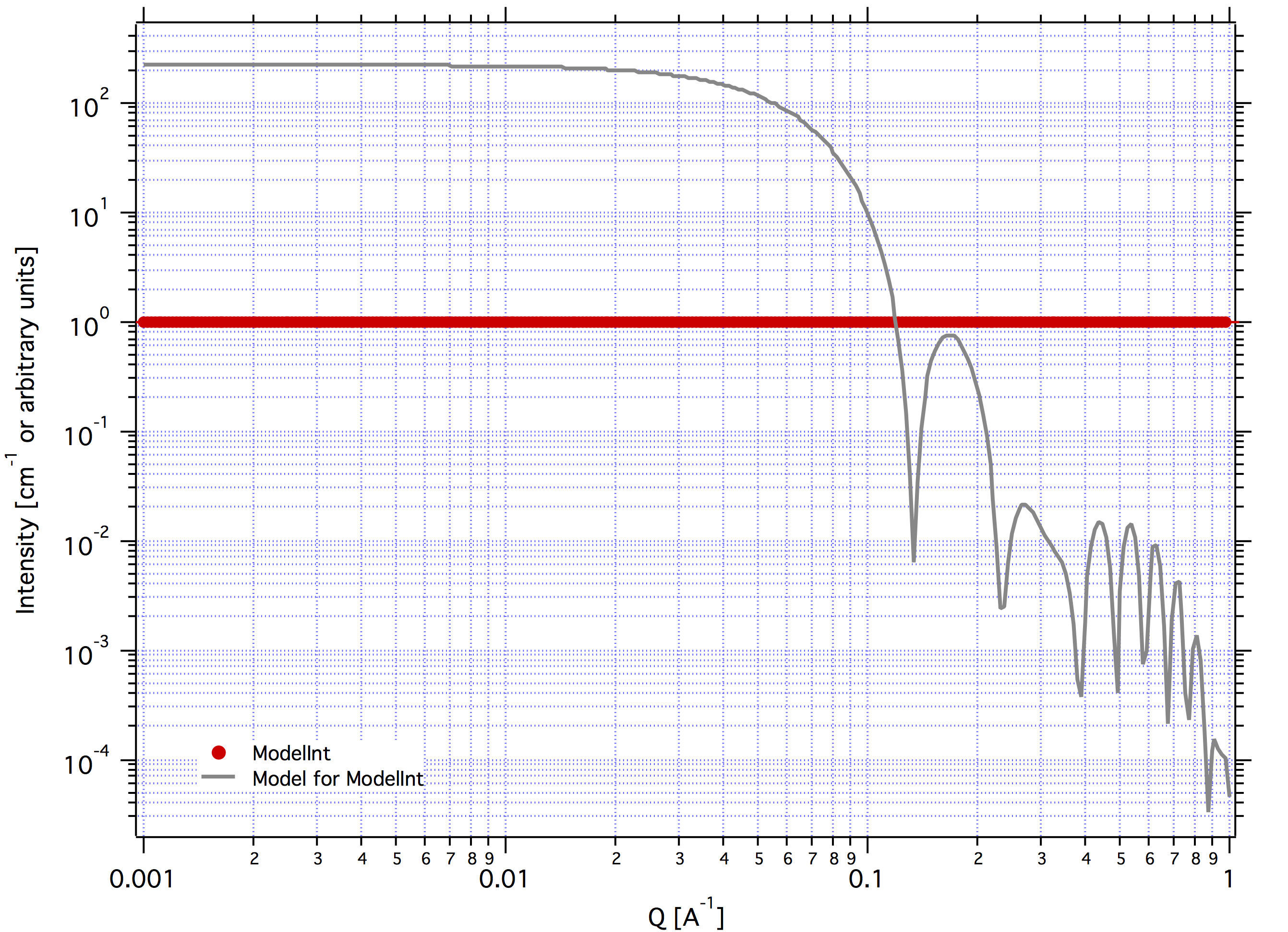
This is graph of NIST model and Irena implementation.

../_images/StructureFactor_HardSpheres.png

StickyHardSpheres¶

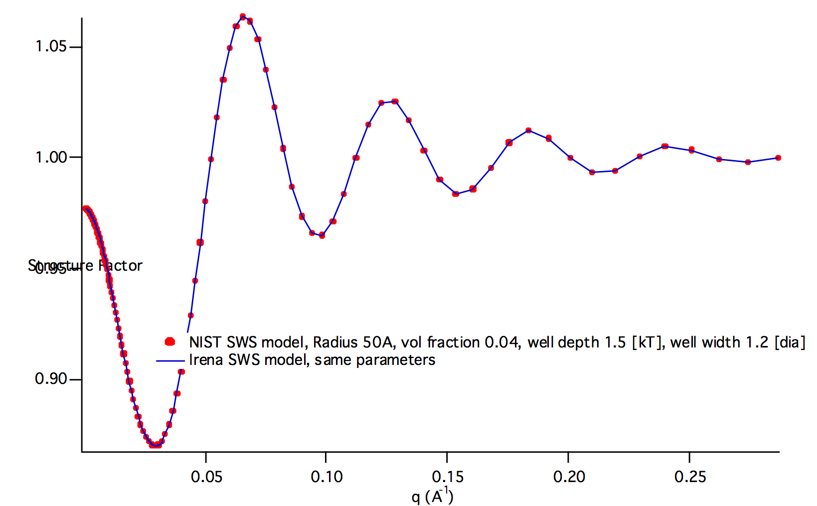
SquareWell¶

HayerPenfoldMSA¶

The code for this structure factor has been copied from NIST SAS macros (Kline, S. R. (2006). For any details on the use of these, please see the original code and description from NIST data analysis package (http://www.ncnr.nist.gov/programs/sans/data/data_anal.html)Åc Please, give them credit when using this structure factor.

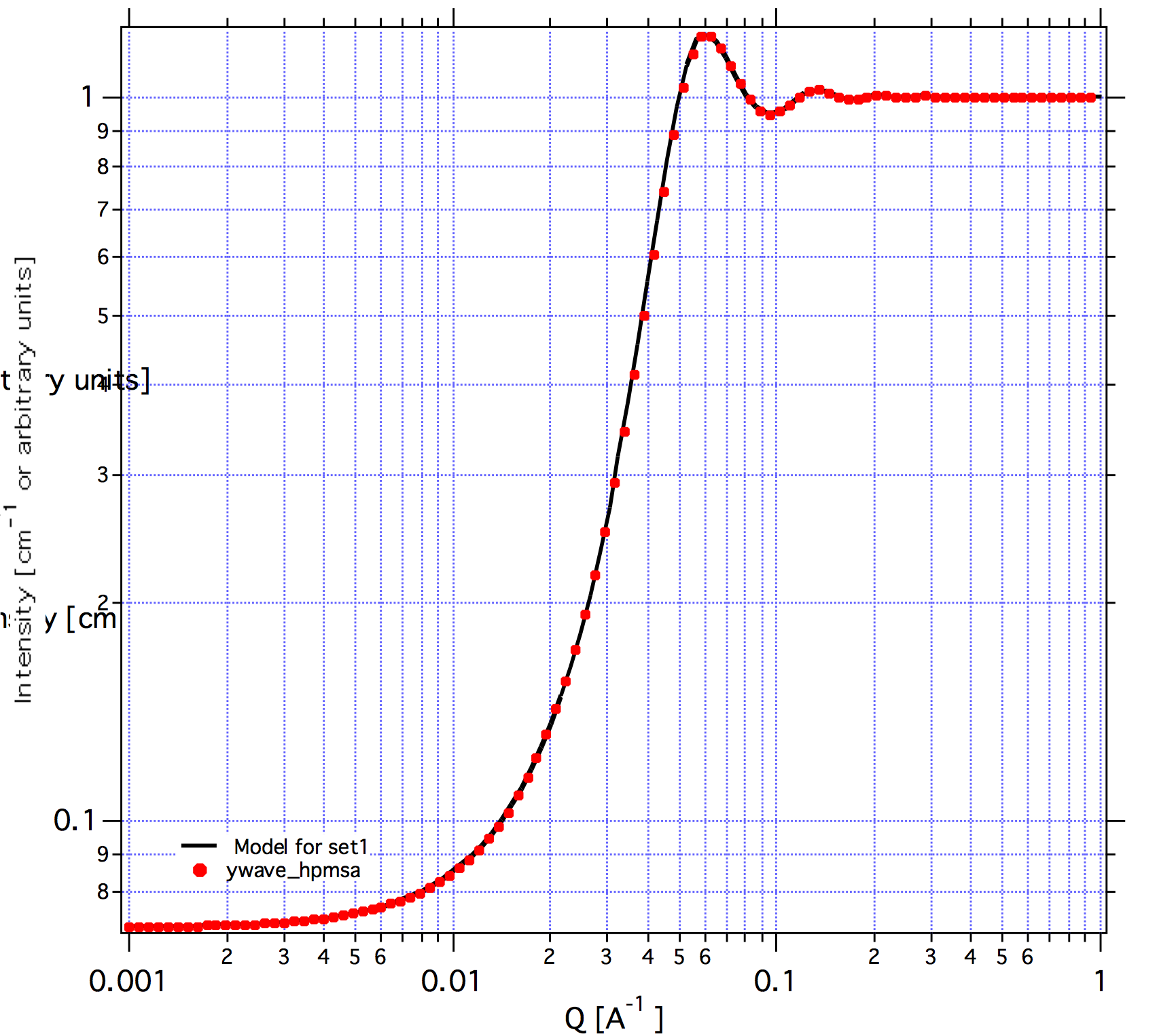
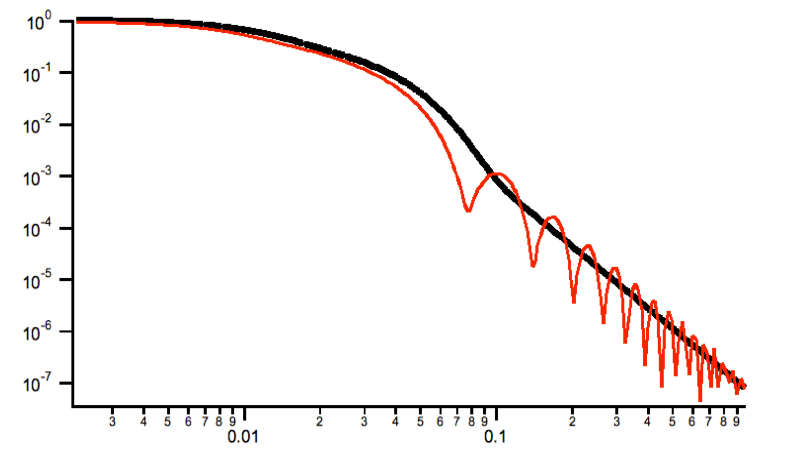
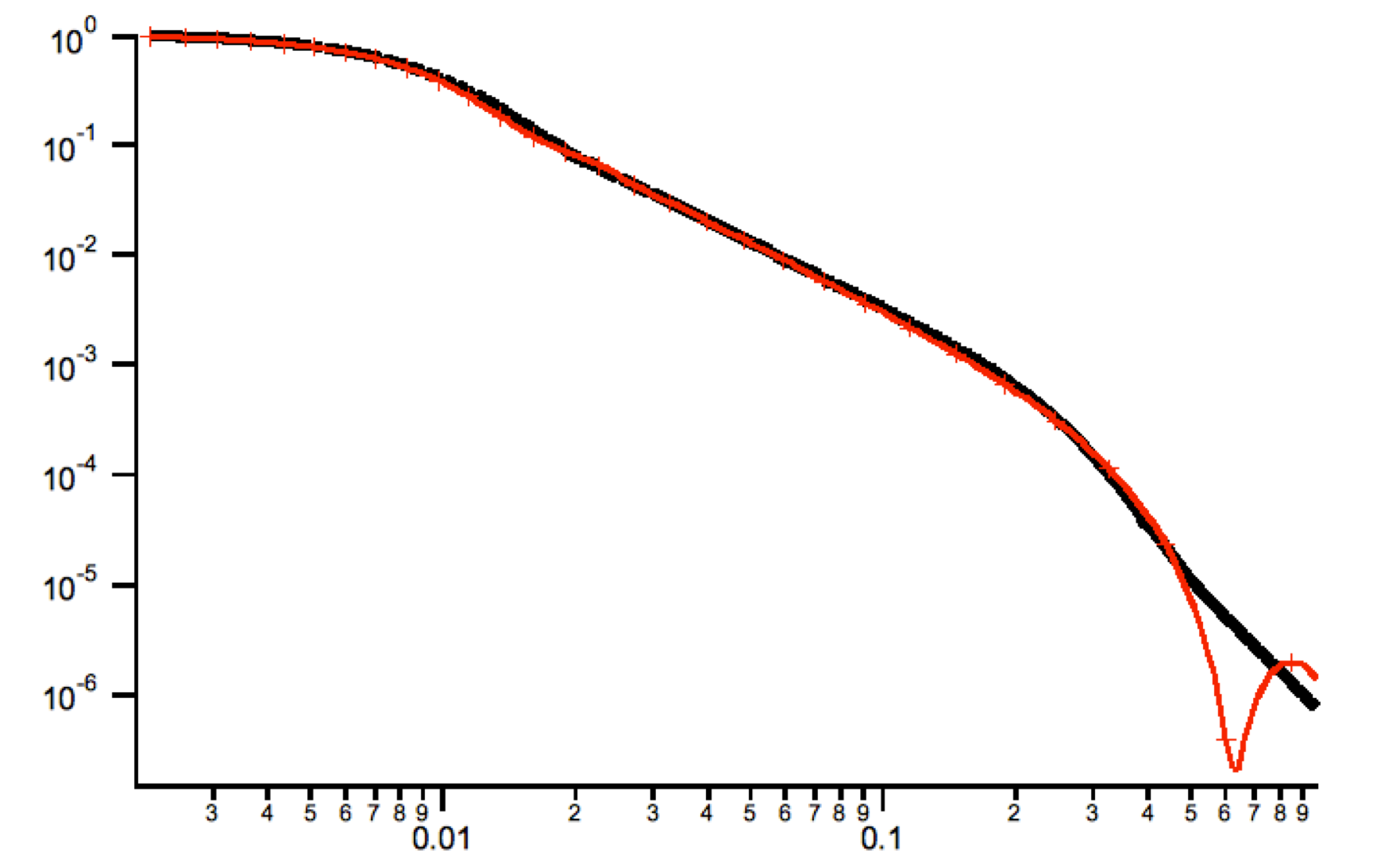
This is graph fro standard NIST set of parameters for both Irena package (black line) and NIST package (red dots). Both assume ONLY structure factor (Form factor is set to 1). The parameters were: Diameter (A) 41.5 NOTE: Irena uses here radius, which is converted to diameter inside the structure factor. This is to keep consistency with other structure factors. Charge 19 Volume Fraction 0.0192 Temperature(K) 298 monovalent salt conc. (M) 0 dielectric constant of solvent 78 Units are mentioned in the help for each filed on the Structure factor panel (you may have to enable help on Mac, it is shown always on PC in the bottom left corner of the Igor window). Important note: this is comment from original NIST codeÅc. // * NOTE ** THIS CALCULATION REQUIRES THAT THE NUMBER OF // Q-VALUES AT WHICH THE S(Q) IS CALCULATED BE // A POWER OF 2 //!!!!! this is at this time NOT enforced in Irena implementation... // I am not sure if this is really problem or not. // How do I find out? Users need to test this for me and if necessary, I need to try it out. // in my testing there was NO problem with the results when the number of q pointds was arbitrary number of points...

InterPrecipitate¶

The code for this structure factor has been created on user request for study of precipitation in metals. It is based on formula 6 from APPLIED PHYSICS LETTERS 93, 161904 (2008), Study of nanoprecipitates in a nickel-based superalloy using small-angle neutron scattering and transmission electron microscopy by : E-Wen Huang, Peter K. Liaw, Lionel Porcar, Yun Liu, Yee-Lang Liu, Ji-Jung Kai, and Wei-Ren Chen. This manuscript refers for this formula to paper by R. Giordano, A. Grasso, and J. Teixeira, Phys. Rev. A 43, 6894 (1991). I did not look up original reference, so check it youself to make sure theformula is OKÅc

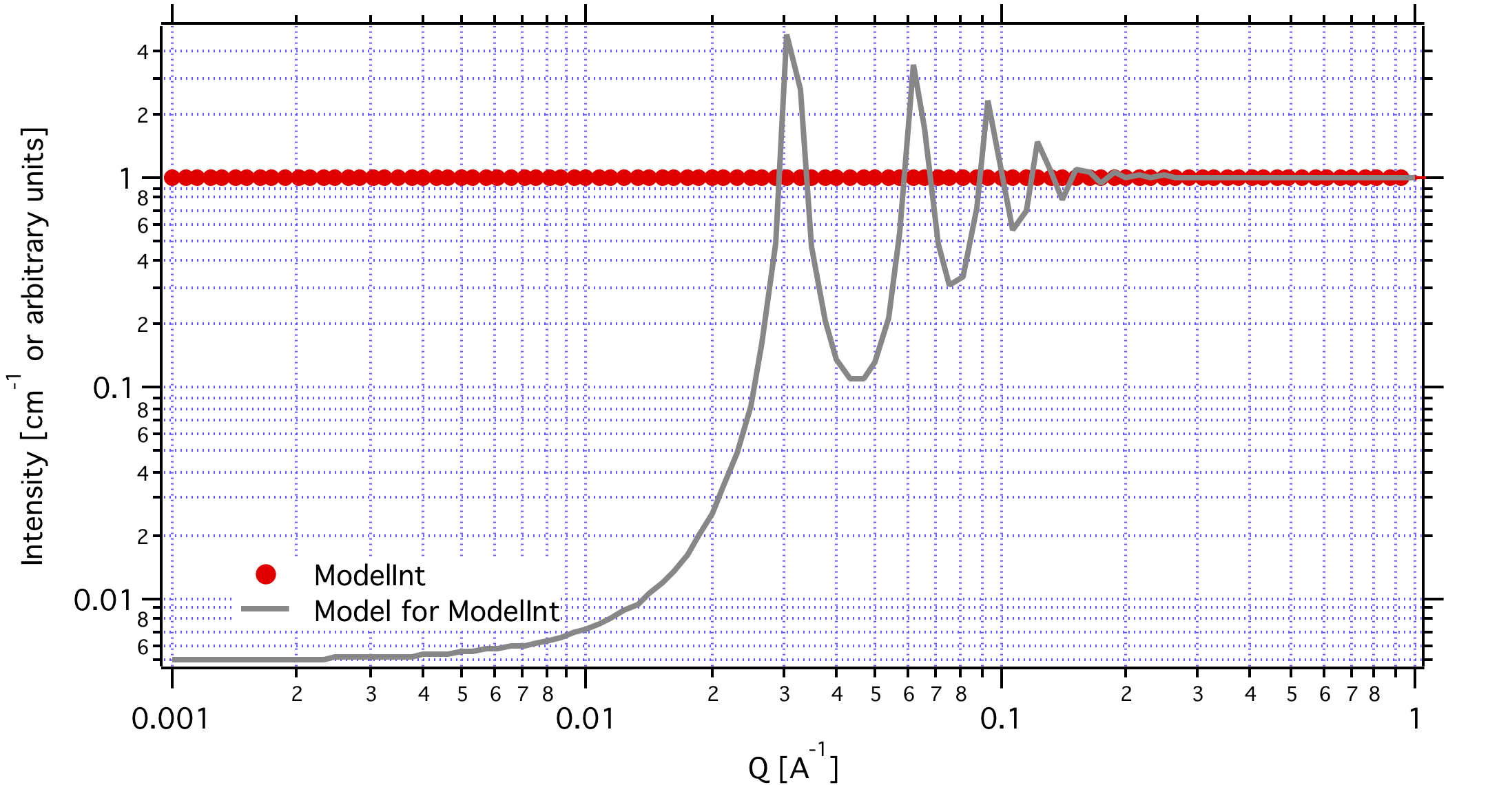
Structure factor has two parameters - L distance and sigma - root-mean-square deviation (ordering factor):

In Igor code this is programmed:

top = 1 - exp(-(Q^2*sigma^2)/4)*cos(Q*L) bot = 1-2*exp(-(Q^2 * sigma^2)/4)* cos(Q*L) + exp(-(Q^2*sigma^2)/2)

S(Q,L,sigma) = 2*(top/bot) - 1

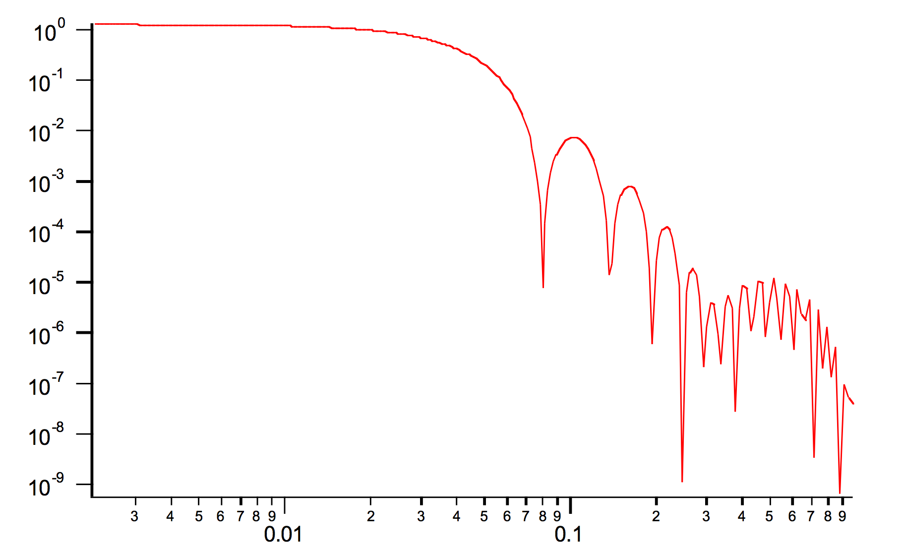
This is model of the SF for L=200 and Sigma=20 (Sigma/L=10). I have no way of testing this so this formula has not been checked against any data.

Calling the library and use¶

Users can use built in library in their own code using following calls:

initialize by calling: IR2S_InitStructureFactors()

this is where the list of known structure factors is: SVAR ListOfStructureFactors=root:Packages:StructureFactorCalc:ListOfStructureFactors
use by calling: IR2S_CalcStructureFactor(SFname,Qvalue,Param1,Param2,Param3,Param4,Param5,Param6)

I(Q) = I(Q, dilute limit) * IR2S_CalcStructureFactor(SFname,Qvalue,Param1,Param2,Param3,Param4,Param5,Param6)

//Dilute system;Interferences;HardSpheres;SquareWell;StickyHardSpheres;HayterPenfoldMSA

3. Get panel by calling: IR2S_MakeSFParamPanel(TitleStr,SFStr,P1Str,FitP1Str,LowP1Str,HighP1Str,P2Str,FitP2Str,LowP2Str,HighP2Str,P3Str,FitP3Str,LowP3Str,HighP3Str,P4Str,FitP4Str,LowP4Str,HighP4Str,P5Str,FitP5Str,LowP5Str,HighP5Str, P6Str,FitP6Str,LowP6Str,HighP6Str,SFUserSFformula)

to disallow fitting of parameters, simply set FitP1Str=”” etc.

then do not have to set low and high limits ...

Structure factors package... IR2_OldInterferences this is roughly hard spheres (close to Percus-Yevick model, not exactly), the ETA = 2* radius and Phi = 8 * vol. fraction for PC model. IR2_HardSphereStruct this is Percus-Yevick model IR2_StickyHS_Struct this is sticky hard spheres IR2_SquareWellStruct this is Square well IR2_HayterPenfoldMSA this is HayterPenfoldMSA IR2_InterPrecipitateSF this is InterPrecipitate