Mass Fractal Aggregate model

This tool generates 3D model RANDOM representation (voxelgram) of Mass fractal aggregate. For details on the science behind it see paper : A. Mulderig et.al., Quantification of Branching in fumed silica, J. of Aerosol Science 109 (2017) 28-37, http://dx.doi.org/10.1016/j.jaerosci.2017.04.001

This tool is applicable ONLY to mass fractals It is critical users understand its limitations and the meaning (and reliability of) mass fractal aggregate parameters as used in the tool. These are listed below.

This is “visualization tool” - it is NOT fitting of data. Data are first fitted by Unified fit and, assuming users have mass fractal, fractal parameters describing the Mass Fractal system they have are calculated. Users then can use this tool to RANDOMLY generate one or more mass fractal aggregates. That is: user generates using Monte Carlo method each time one of MANY possible shapes of this mass fractal. If the mass fractal shape has same or similar fractal parameters properties it is assumed that it looks similar to what the aggregate inside the sample looks like. So, this is NOT fitting, it is random shape generation and user need to vary model growth parameters until model with suitably similar mass fractal parameters is grown. Once proper growth parameters are found, user can grow number of representative shapes.

Keep in mind, that this is really random process and same growth parameters will result in wide ranging models. One needs to run many times and see, how the results vary. Store results which are close to your target data, you may never recreate them.

Some parts of the code generate randomly errors or failures. I will be trying to find a solution fo those which are errors, some are simply results of random growth. In any case, solution is to run model again. There are some specific conditions which seem to fail all the time. Select different parameters.

Mass Fractal model parameters

Following manuscript: http://dx.doi.org/10.1016/j.jaerosci.2017.04.001

Mass Fractal aggregate has following parameters:

• R - aggregate size
• d_f - Mass fractal dimension of the aggregate
• p - short circuit path length
• s - connective path length
• d_min - minimum dimension of the aggregate
• c - connectivity dimension of the aggregate
• s - connective path length of the aggregate

Each of these terms can be inter-related with each other by:

\[R=\frac{R_g}{d_p}=z^{1/d_f}=p^{1/d_{min}}=s^{1/c}\]

Where:

• Rg is the Radius of gyration of the second (Large) level - represents the size of the mass fractal aggregate.
• d_p is Sauter mean diameter of a sphere of similar surface to volume ratio as the scattering primary particle (first, smaller level).

The value z which is one of the inputs of the 3D aggregate model, d_min, and c are calculated by Unified fit tool in “Analyze results”. The value of d_f is power law slope of the second (larger) level when Mass fractal is represented by two Unified levels.

******

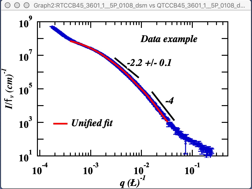
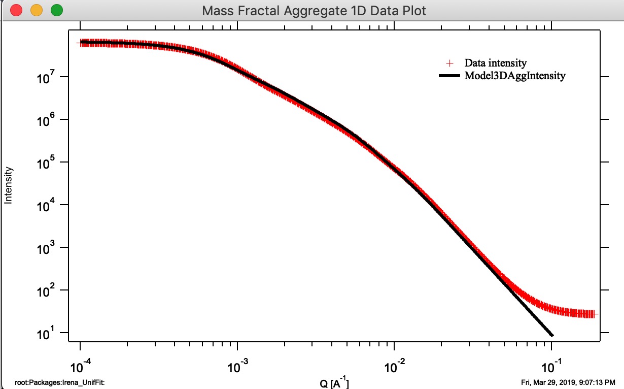
Here is example of data provided by one of the authors of the method and associated Unified fit with two levels. This is mass fractal system, there we have primary particle size (approx. 320A Rg), mass fractal with dimension of ~2.23 and large Rg of about 2332 A.

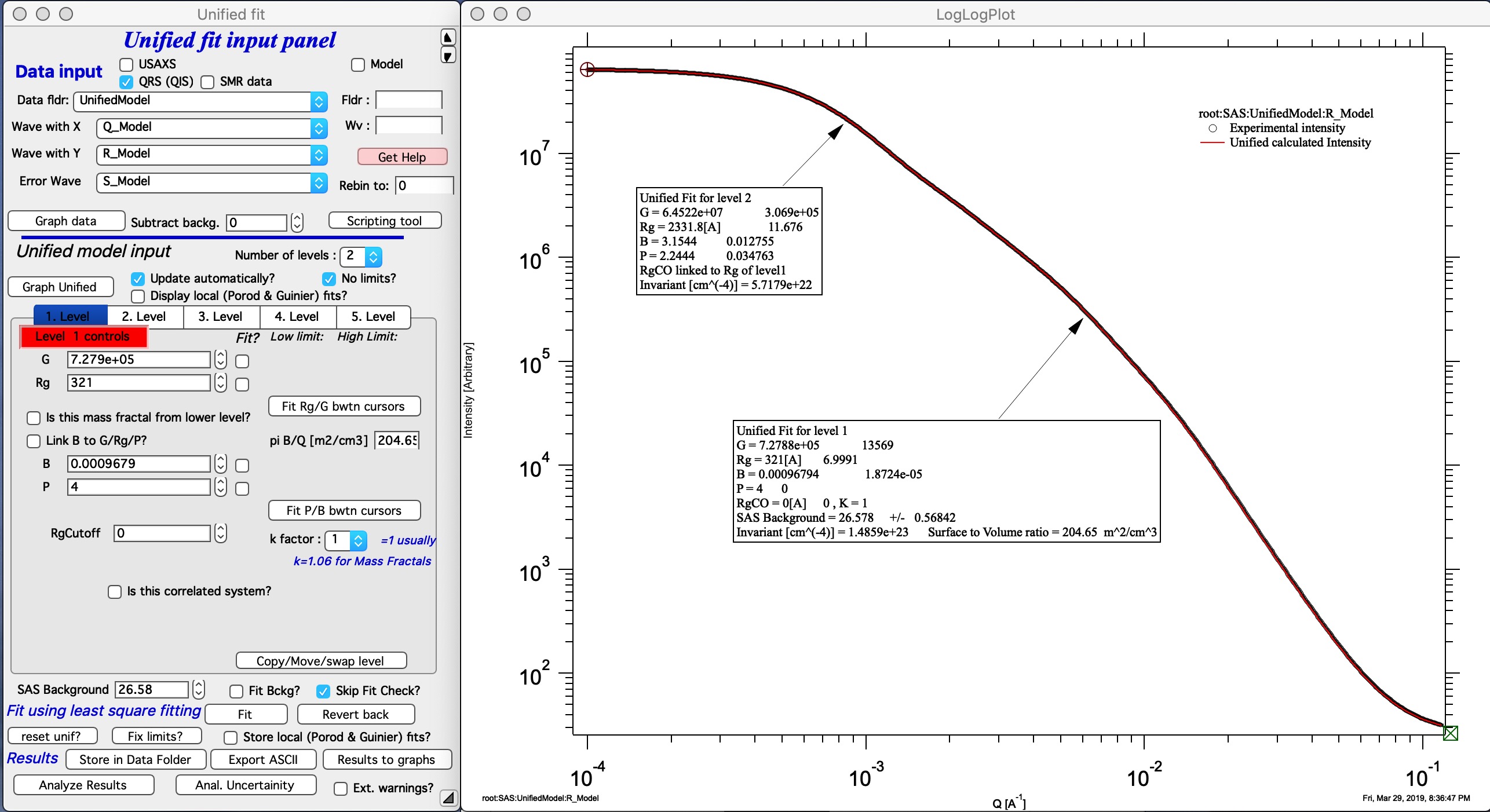
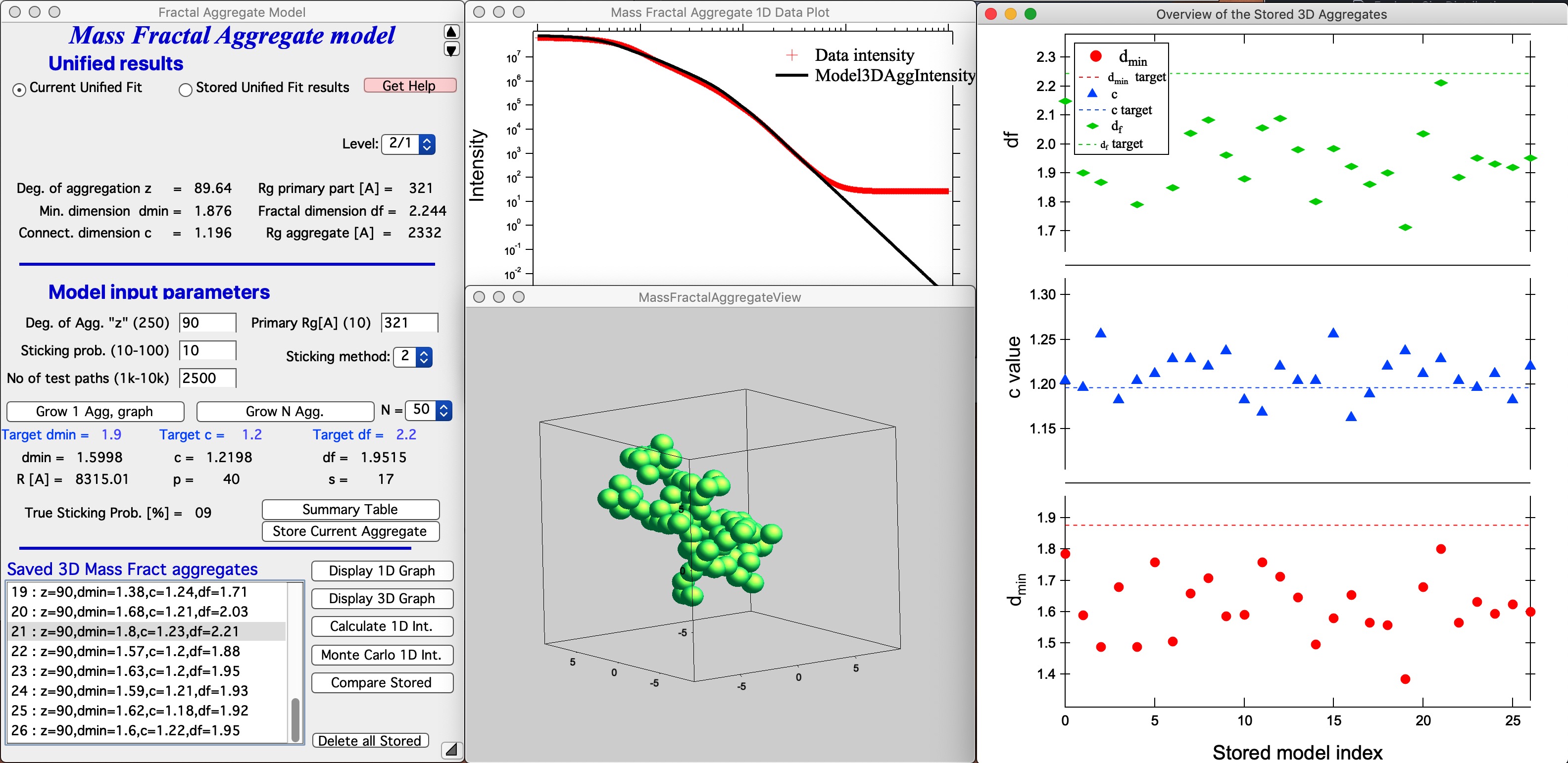
Now, when we have the Unified fit results above, we can either run directly the Mass Fractal Aggregate tool, or first save the results of Unified fit in a folder where the data came from (Store in Data Folder). Important is, that we have needed numbers which will guide our modeling. Here is the main panel:

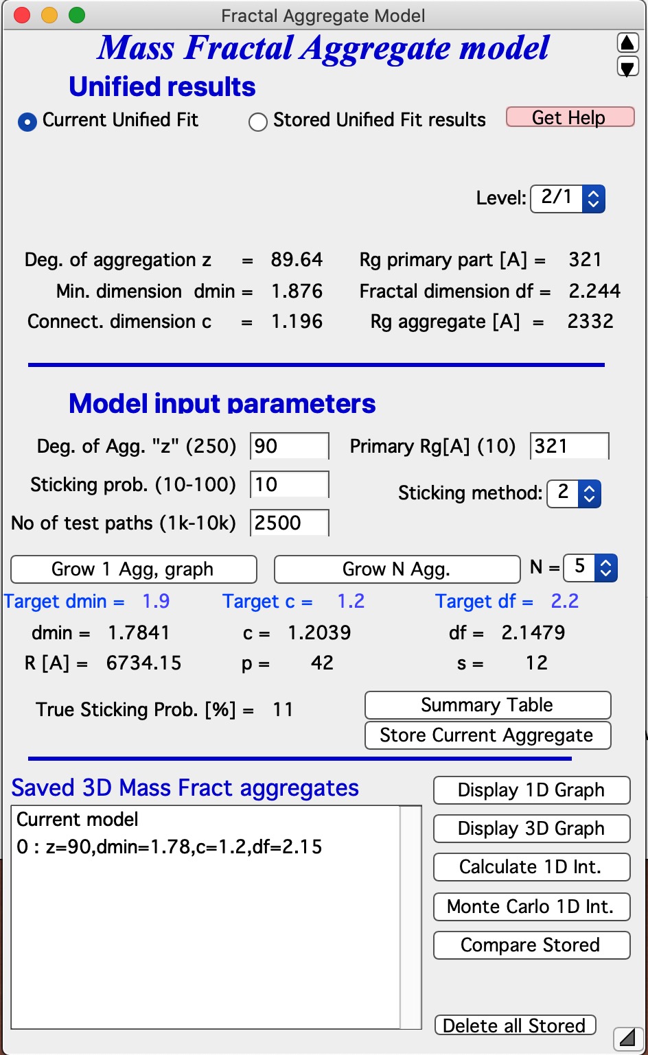
Let me describe the content of this panel: In the top part are options to use results from Unified fit using modified version of standard data selection tools . This is simply lookup tool, user can as well pick the needed numbers from Analyze Results in Unified fit. Data can be selected from Stored Unified Fit results or - as in the picture above - from current Unified fit working directory, using whatever values are in the current Unified Fit tool. This is result of the last Unified fit fit or manual change… By default we assume, that levels 2/1 represent the Mass Fractal, but it can be changed by using the popup “Level” as needed. NOTE: The values are updated after user selects or reselects the Level choices, so if the numbers are stale, just reselect that popup display and values will be updated. Based on these selections, the code extracts needed parameters and presents them in table - and the most useful ones are repeated below the “Grow Aggregate” in blue color. These are your target values, what your aggregate should have to represent the Mass fractal scattering.

The most interesting are z = degree of aggregation and d_f

The parameters user uses to control growth are:

• Degree of aggregation “z” - this is how many particles will be in the aggregate.
• Sticking probability - this is probability of sticking in the Monte Carlo method - when a new particle arrives nearby any existing aggregate particle, how likely it is to stick. Value varies from 10 to 100%.
• Sticking method. There are three values here 1, 2 and 3. Sticking method describes how close must a new particles arrive to existing ones to be allowed to stick. These distances relate to which neighbor it needs to be within the system which is simple cubic lattice, which is used to move particles around. 1 is really nearest neighbor in one direction only (x or y or z direction only), 2 is neighbors include also in plane neighbors (xy, xz, etc), and 3 are neighbors also in body direction (including xyz neighbor). Value of 3 allows particle to stick if it is relatively far from any aggregate particle (distance of sqrt(3)), value of 2 means it has to be closer (distance of sqrt(2)) and 1 means it has to arrive really close (distance of 1).

Using different combinations of sticking probability and Sticking method results in different structures. And of course, as any proper Monte Carlo method, results are random… User needs to test various combinations to find a combination which creates aggregates which have parameters which match parameters of his/her scattering.

Note: lower Sticking probability and larger z values significantly increase run time. Watch history area where progress is presented and final parameters are listed also.

NOTE : growth of aggregate can fail if too compact particle is grown. When this happens, simply try again.

No of test paths This is internal parameter which is defining how many different attempts to pass through the aggregate code does to calculate the resulting parameters. Higher number results in better statistical validity of the numbers for c, d_f, d_min, etc. But takes longer time. 2.5k seems kind of good compromise.

Primary Rg[A] This gives the whole aggregate real size - copy here size of primary particle Rg.

Grow the particles:

OK, now we can grow the particles. First try growing one particle - see next button - and if all works as expected, grow multiple particles (and go and get coffee, it may take some time). Note, that this is CPU intensive calculation.

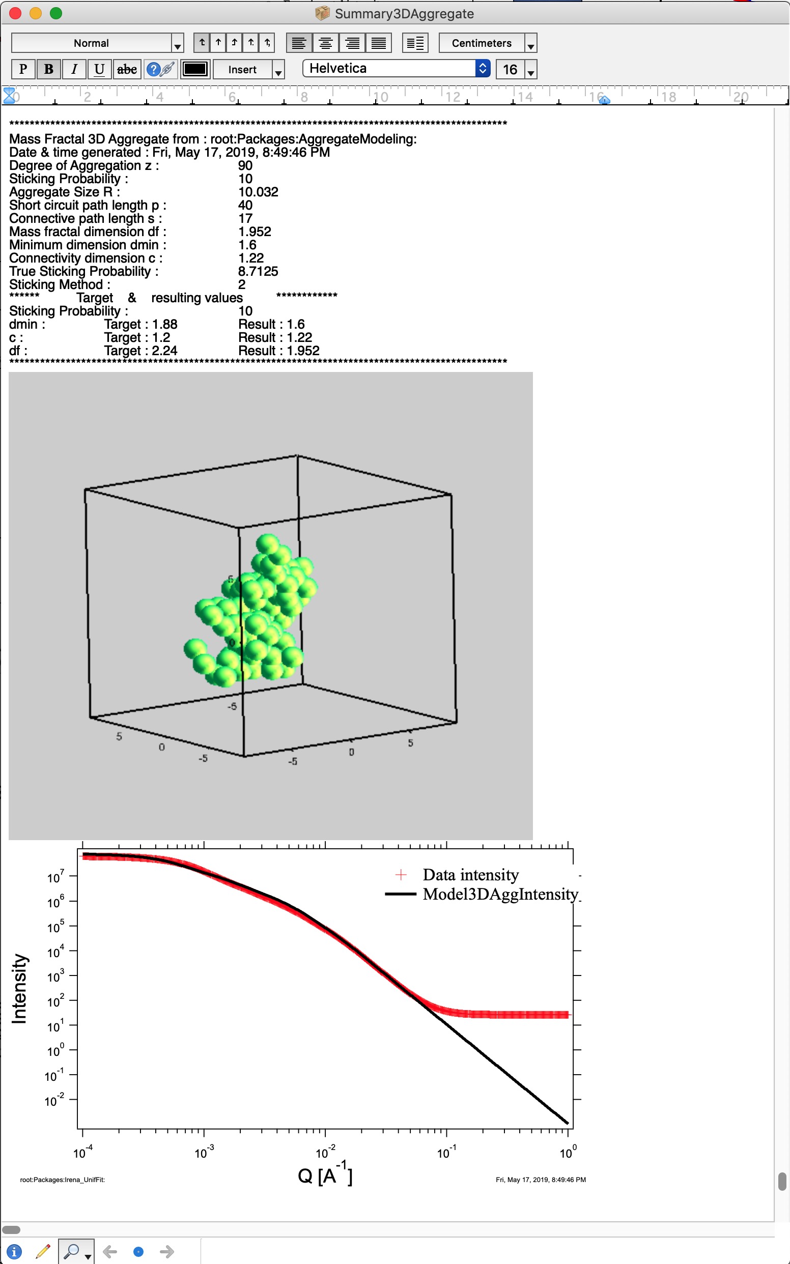
This MAY BE SLOW Push Button “Grow 1 Agg, graph” and this will create the aggregate and display it in Gizmo as well as calculate 1D intensity data and overlay them over the data from source folder. Below is result which run on my high-end MacBook Pro for about 15 seconds:

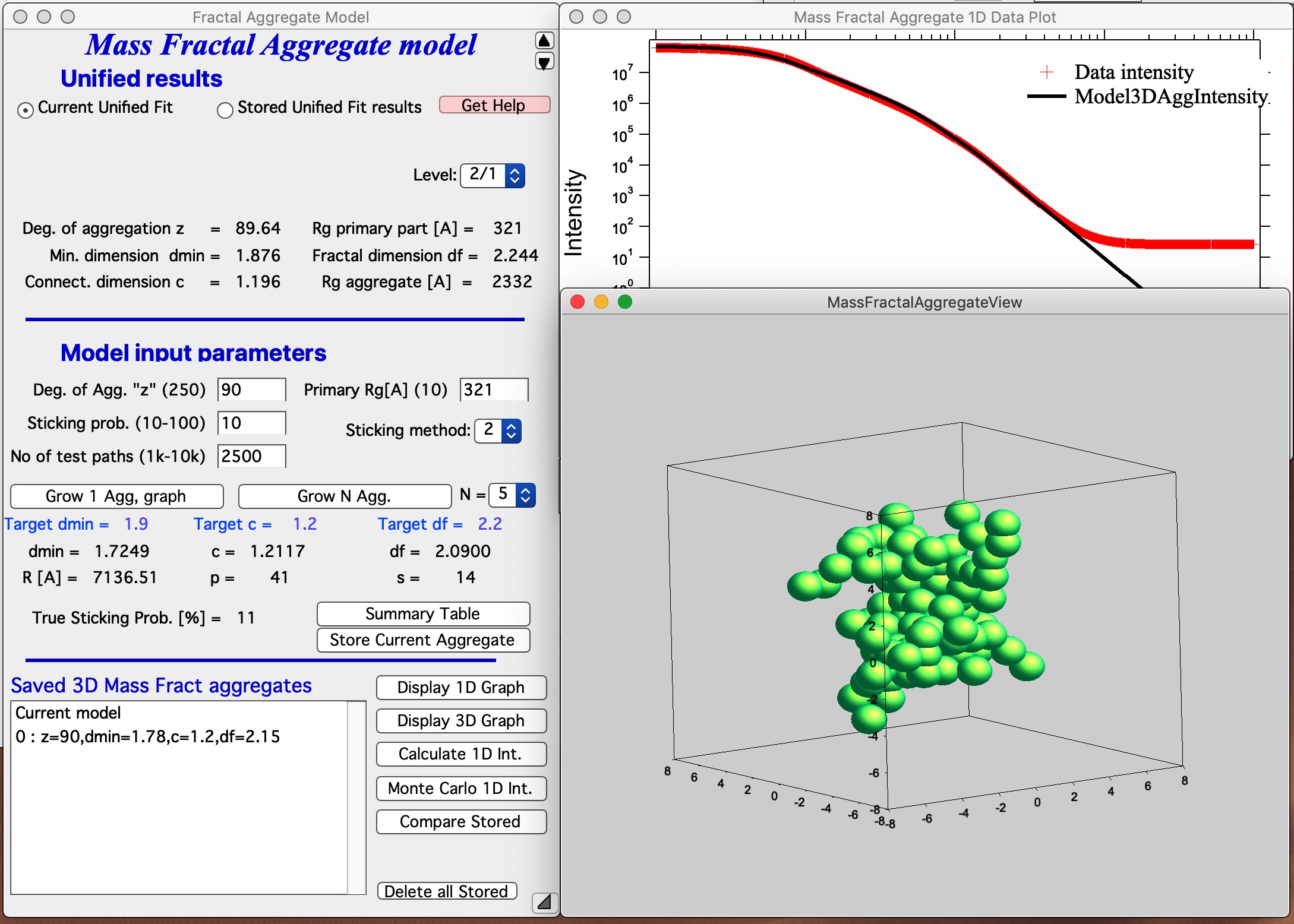
This is relatively good result. It is unlikely that all parameters will be matched exactly - or even very close. Note in the first graph with data the slope (d_f) has uncertaintiy of 0.1, it is unreasonable to try to match this value more precisely. It may be useful to use “Analyze uncertainties” in Unified fit to understand the precision with which the parameters are known. I have d_f of about 2.09 (and need 2.2); c about 1.21 (and need 1.2); and d_min about 1.72 (and need 1.9). I think this is close to acceptable for this model. Also note, that the fit in the 1D intensity vs Q is reasonably good.

This WILL BE SLOW Push Button “Grow N Agg” and this will create N aggregates sequentially (N is selected in the pull down menu next to this button, default is 5, max is 50), display it in Gizmo as well as calculate 1D intensity data, overlay them over the data from source folder, save the aggregate and store achieved results in notebook. These results can be the evaluated using button Compare Stored, see below.

NOTE : When too compact particle is grown, it is skipped and nothing is saved. It is therefore common, that you end up with less than N saved aggregates to evaluate.

Button “Summary Table” displays Notebook with model summaries - and adds in there current results summary, see below. This can be used to follow how results depend on model input parameters and make notes. See below image for a record from one model run. This record needs to be created manually when growing one aggregate, but is created automatically, when growing N aggregates.

Button “Store Current Aggregate” stores the current aggregate result (including the 3D aggregate data) in separate folder, where they can then be found, displayed etc. It also adds results into the ListBox Saved 3D Mass Fract Aggregate, see list in Listbox below. I just added there the current result. Description in the table describes resulting parameters achieved for that Mass Fractal Aggregate. You can then select a line and generate 3D and 1D graphs etc.

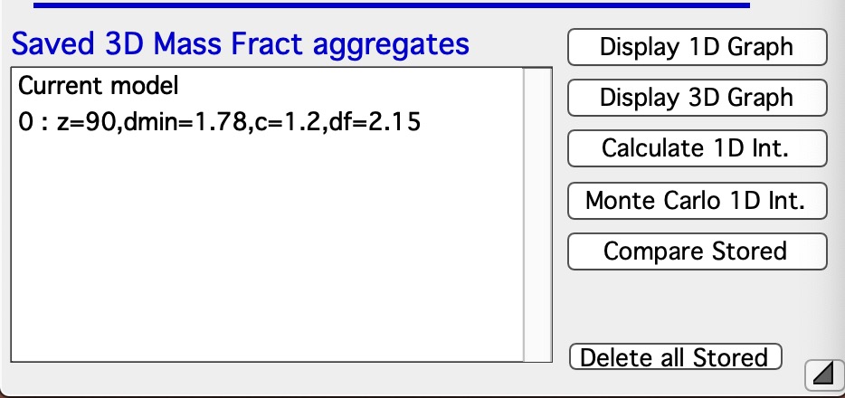
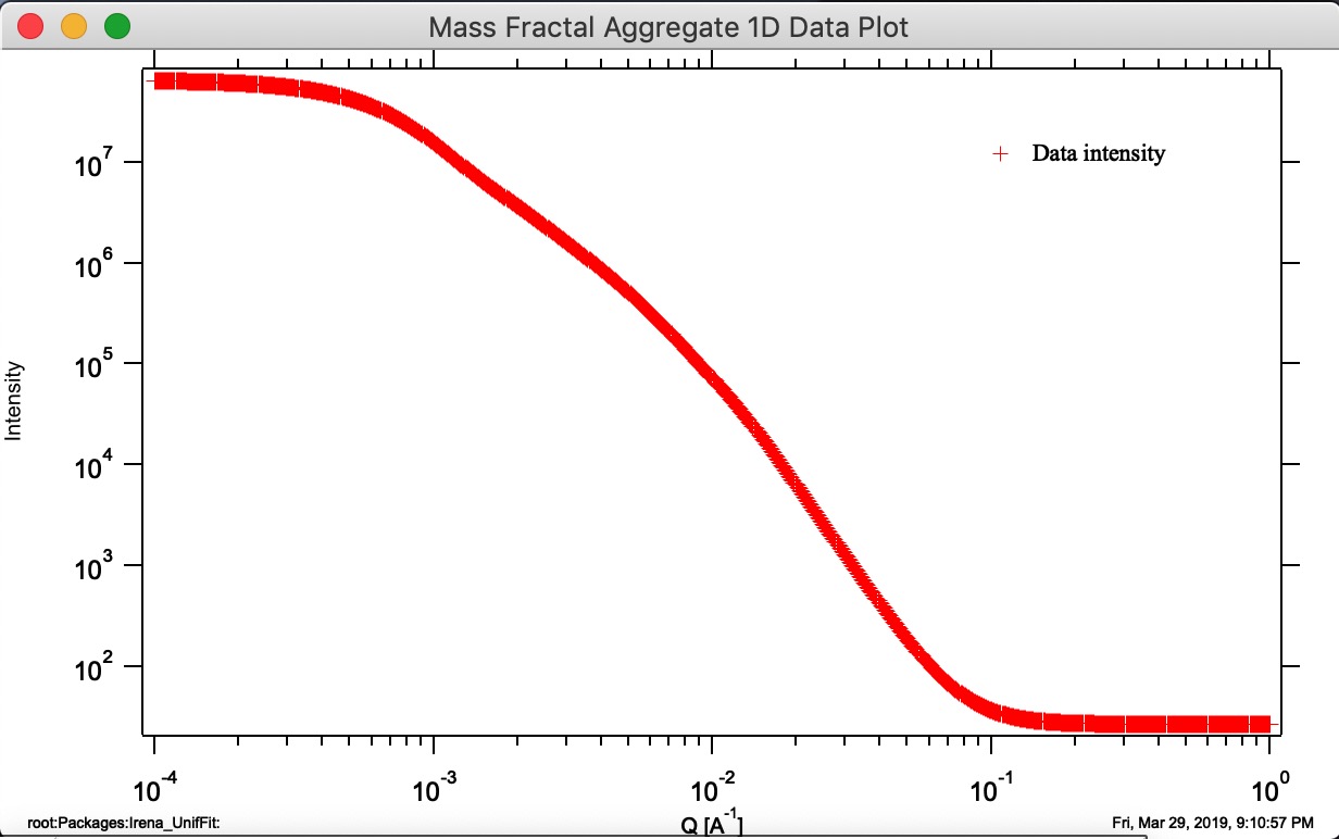
Button “Display 1D graph” Pulls Int/Q data from folder where parameters came from and creates a new graph (“Mass Fractal Aggregate 1D Data Plot”). Note, does not append any model data, for that you need to push buttons Calculate 1D Int. and/or Monte Carlo 1D Int.

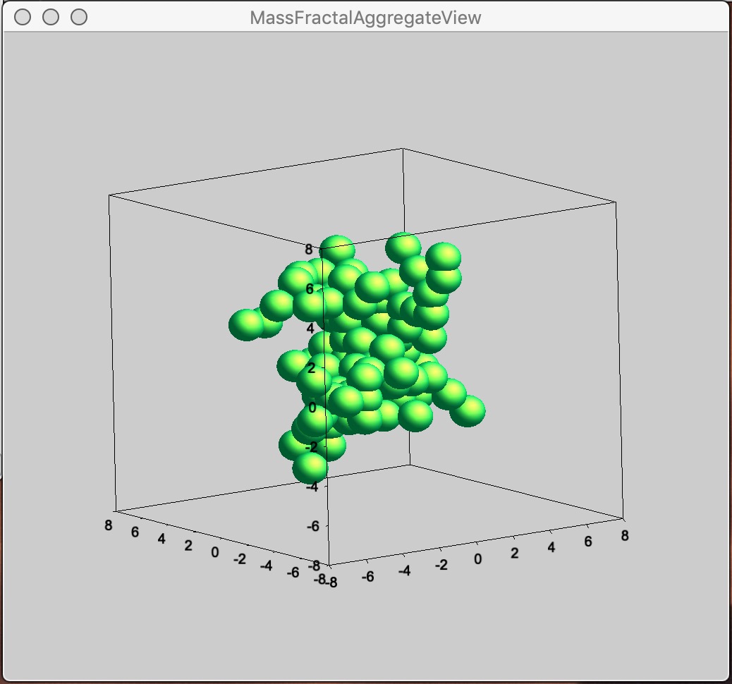
Button “Display 3D graph” Displays in the Listbox selected Mass Fractal result in Gizmo. If nothing is selected, current result in working directory (if exists) is presented.

Button “Calculate 1D Int.” Calculates 1D intensity of the Aggregate based on its parameters and appends the calculated intensity of the aggregate to “Mass Fractal Aggregate 1D Data Plot”. Model data are matched to measured data using area under the curve over middle part of the q range, where curves are likely to overlap. Keep in mind, this model predicts SHAPE of the 1D curve, not absolute intensity, of course…

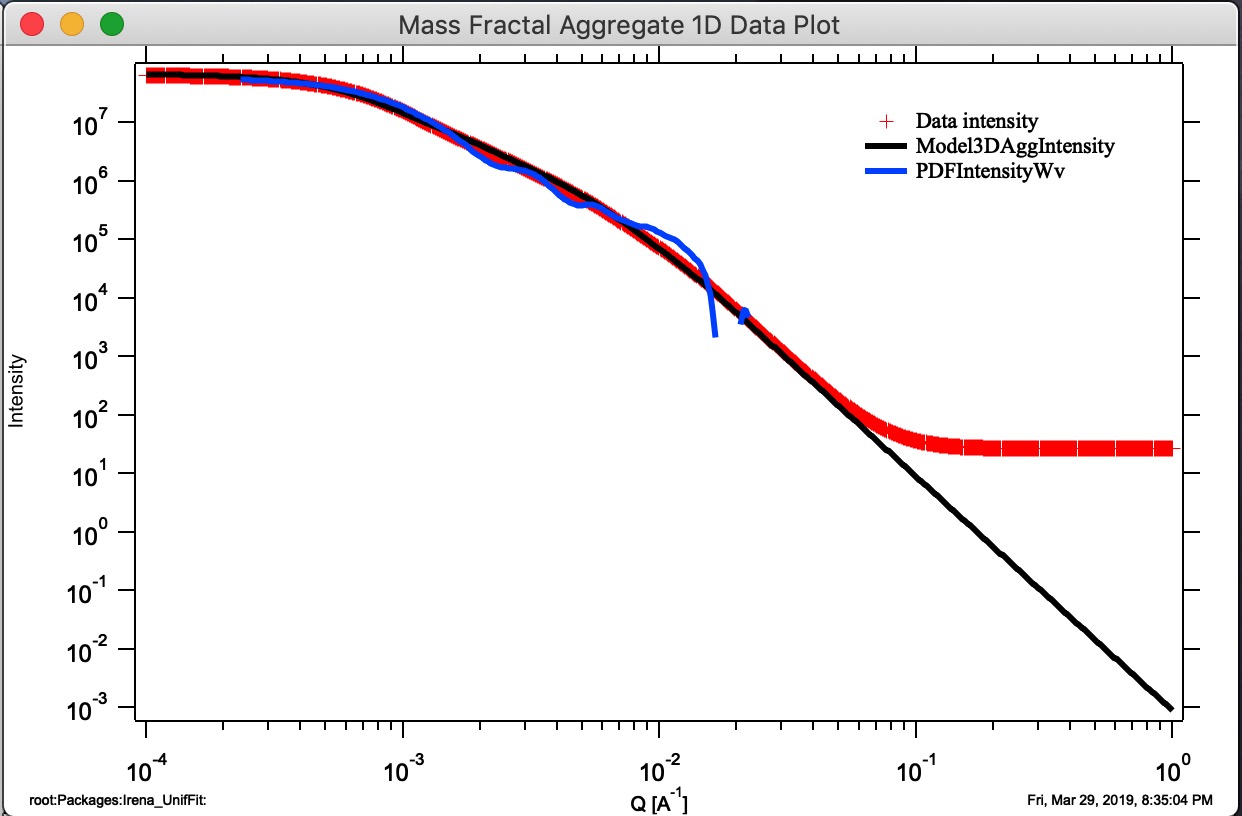
Button “Monte Carlo 1D Int.” Calculates 1D intensity of the Aggregate using Monte Carlo method and appends the calculated intensity of the aggregate to “Mass Fractal Aggregate 1D Data Plot”. This is not working very well and takes a long time. Also, for numerical reasons and really poor sampling, the results are noisy and not very representative of higher Q values, see graph below - the blue curve is calculation using Monte Carlo calculation of PDF and conversion into Intensity vs Q. It is kind of close and really nice it proves the model matches the data, but not very helpful. I suggest users to ignore it for now…

Button “Compare Stored.” If users run multiple aggregate growths (either manually or using Grow N Agg. button), thy may have many different aggregates stored. This is Monte Carlo method, so each time we run the model, we get slightly different result. It is therefore critical to be able to somehow evaluate which one is closest to the target parameters. This button will plot three main parameters of all saved aggregates to enable comparison. Note the numbering of the folders for easy navigation.

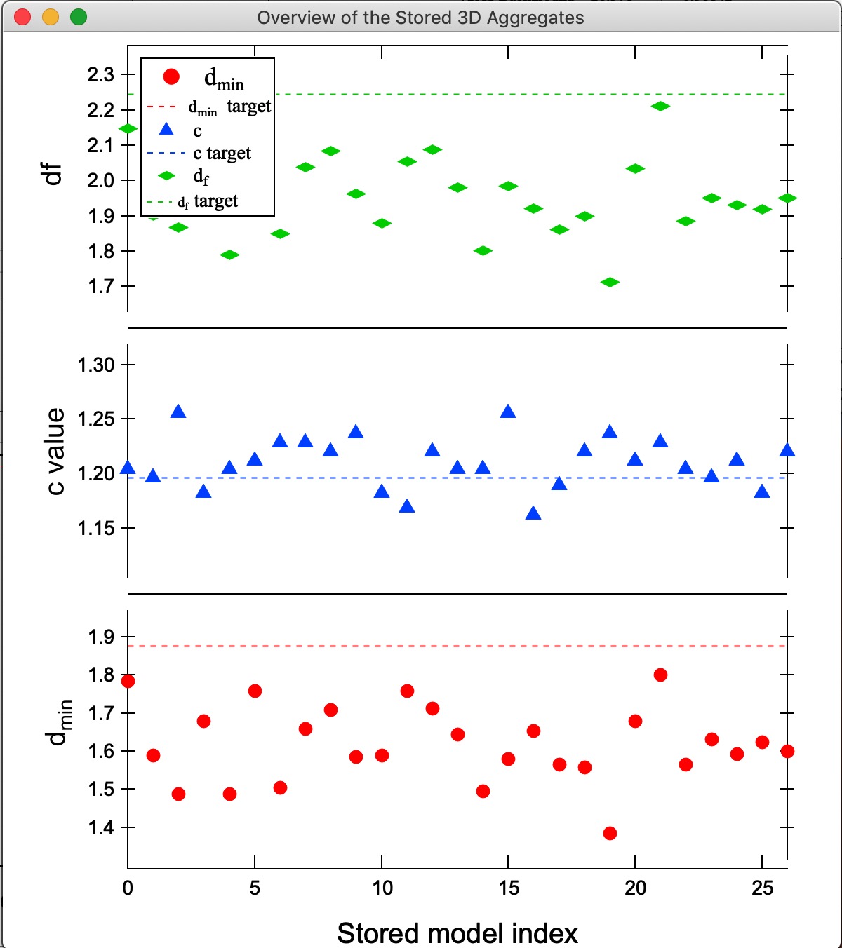
In this plot one can easily see, that while most model match value for c, model 21 is closest for d_f and d_min. We can then select the model 21 in the Listbox Saved 3D Mass aggregates and generate 3D and 1D models of it using the buttons. Here is the best result we got at this time:

Button “Delete all Stored” This button will delete ALL stored 3D Aggregates. It also closes all graphs for this tool to be able to delete these stored aggregates.