Slit smearing in Irena

Slit smearing is built in Irena and is transparent in most of the tools except:

• Guinier-Porod model which seems to be impossible to setup with local fits when using slit smeared data. I have disabled slit smearing in this tool altogether as it was nightmare to use.
• Unified fit. This one allows use of slit smearing fine, but when you do local fits (Power law fit mainly) the fit values are pinhole equivalents. It usually works fine, but gets bit confusing.
• Modeling. Here slit smearing works just fine, but if you use Unified level, local fits also result in pinhole equivalents which is bit confusing.

Smearing of model is intended to work mainly with APS USAXS data - that is with, as described below, approximation of rectangular one dimensional slit. For APS USAXS the slit width is very small (0.00008 1/A) and then one can approximate this geometry as purely slit smeared with only slit length and assume infinitely small slit width. Also, we can assume the slit shape is rectangle as in the Figure below. If this is not satisfied, one needs to desmear the data and used desmeared data in Irena (and use setting for regular, pinhole like data).

We have verified the function of this method by collecting data from the same sample using both slit-smeared and 2D collimated USAXS. We have verified this method repeatedly and every time the slit smearing was blamed for artifacts and unexpected results, we have found another reason for problems. Since desmearing is always going to increase noise on the data, it is usually preferable to fit slit smeared data directly with model with slit smearing included, instead of desmearing the data… Note, that data with absolute intensity calibration are handled correctly.

However, keep in mind that slit smearing and desmearing procedures make assumption of isotropic scattering from the sample, so if samples scatter anisotropically, use of slit smeared data - and slit smeared instruments in general - should be strongly discouraged.

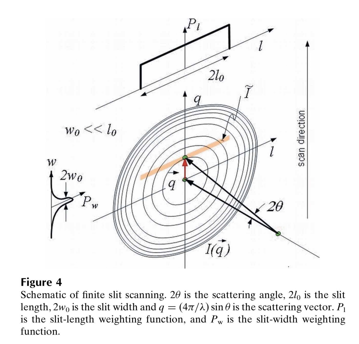
The Figure 4 from J. Appl. Cryst. (2009). 42, 469–479, doi:10.1107/S0021889809008802 shows the definition of slit smearing geometry definition used in this manual. First note, that the smearing is by finite slit length and optionally finite slit width. Slit length is perpendicular to high-q resolution direction (perpendicular to the vertical q direction in figure above). Detector total horizontal opening is actually 2 x Slit length. Slit width is perpendicular to the q direction and is given by detector system (= instrument hardware). Again, total detector opening in the q direction here is 2 * Slit width.

NOTE : Slit length is NOT q-resolution. Slit width actually could be considered q-resolution of the instrument and is sometimes presumed that way. But while slit width is something given by instrument geometry and detector system, final data q-resolution may be lower due to data processing, binning, etc. It can get bit confusing to users. But, slit length assumed in Irena is always perpendicular to the q-resolution direction. Also, Indra and Nika packages produce dQ values and those represent final post-processing q-resolution, which includes effects of slit width combined with data handling, averaging, etc. Therefore dQ exists for Slit smeared data and can be much worse than slit width of the original instrument! Do NOT confuse these two “resolution” values…

Desmearing

Desmearing routine built in this package is using Lake method (reference), which has been originally programmed by Pete Jemian and then coded in Igor by me. There were some minor improvements over the years, but generally this method has proven itself many times to be robust and reliable. We have verified the function of this method by collecting data from the same sample using both slit-smeared and 2D collimated USAXS. We have verified this method repeatedly and every time the desmearing was blamed for artifacts and unexpected results, we have found another reason for problems. That said, desmearing is always going to increase noise on the data… Note, that the routine will correctly handle data with absolute intensity calibration.

This tool, however, allows both slit length (in direction perpendicular to the q direction) and slit width (in direction parallel with q direction). Further, the slit can have shape of trapezoid, similar to what GNOM allows for instrument geometry. PLEASE NOTE: for historical reasons the parameters for Irena desmearing are ½ of the GNOM parameters.

This is the graph:

top side of the trapezoid is 2* slit length – 2*slitLengthL

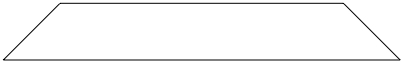
bottom part of the trapezoid is 2* slit length + 2 * slitLengthL

The height of the trapezoid is slit width. Once more, if you have parameters used for GNOM, you have to divide the numbers by ½.

The GUI use of parameters should be easy. Please note, that :

1. If you set slit length or slit width to 0, you assume infinitely high resolution in that direction.
2. If you set “L” parameter to 0, you assume the shape is rectangular in that direction, not trapezoidal.

Theory behind the Desmearing Procedure : See the Lake paper.

Example of the Desmearing Procedure

I have included a file with an example data set with slit smeared data (smeared data.dat) where the slit length SlitLength=0.05113. You can import the data this in your experiment using Data import tool…

Comment – if you need to go back in the routine, anytime you can click on previous tab and return to that place… All from tabs to the right is forgotten and routine restarts on the tab, where you click. It is also possible to skip the smoothing tabs without any penalty – note, that if the smoothing parameters are set (the checkboxes are checked) the data WILL BE smoothed, even when you do not click on the tab…

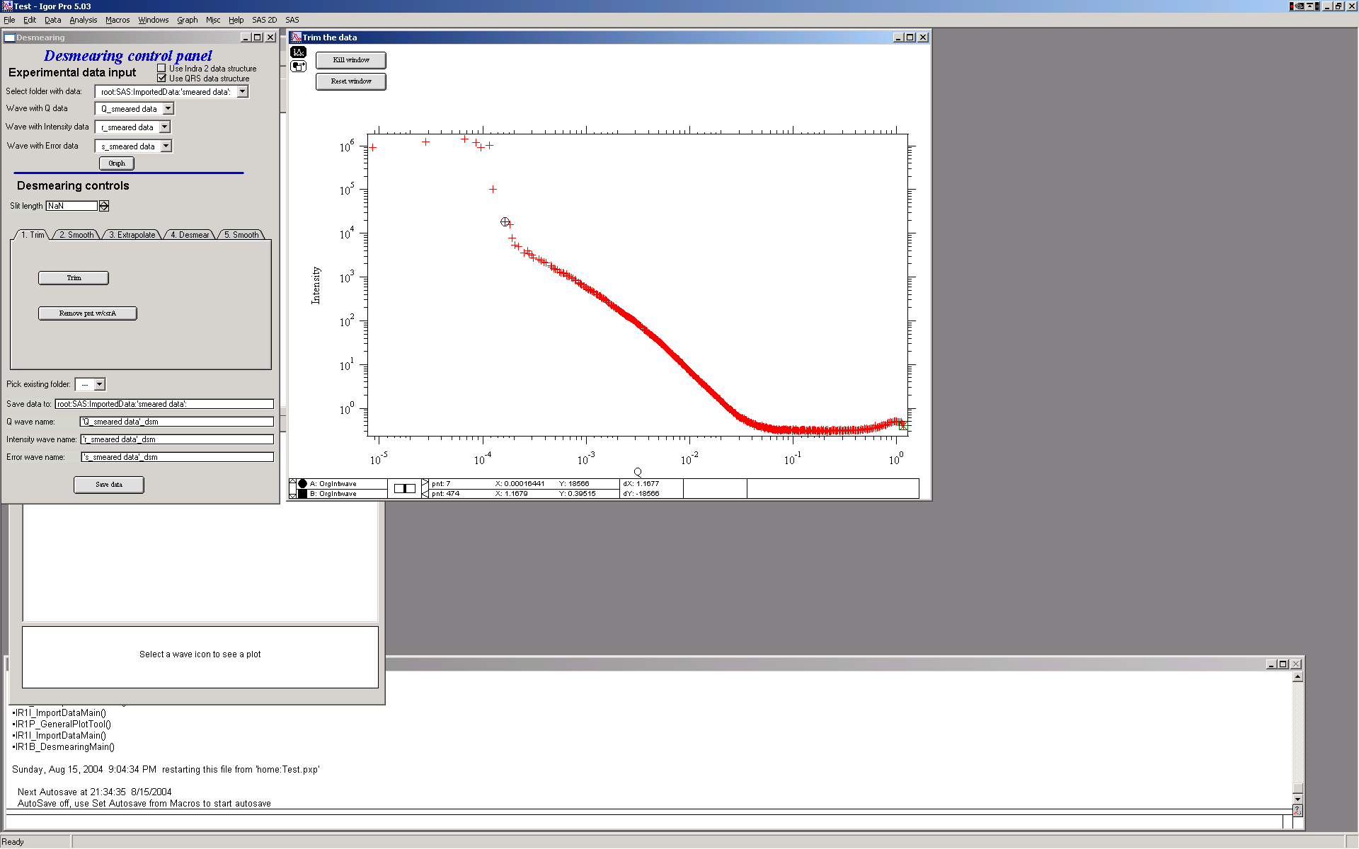
This is GUI and graph after loading data. Only thing needed is to fill in the slit length.

The tool is controlled by the tabs. The order which needs to be followed is the tabs from left to right. For each data set to be desmeared, this procedure must be followed, selecting in sequence the tabs from left to right.

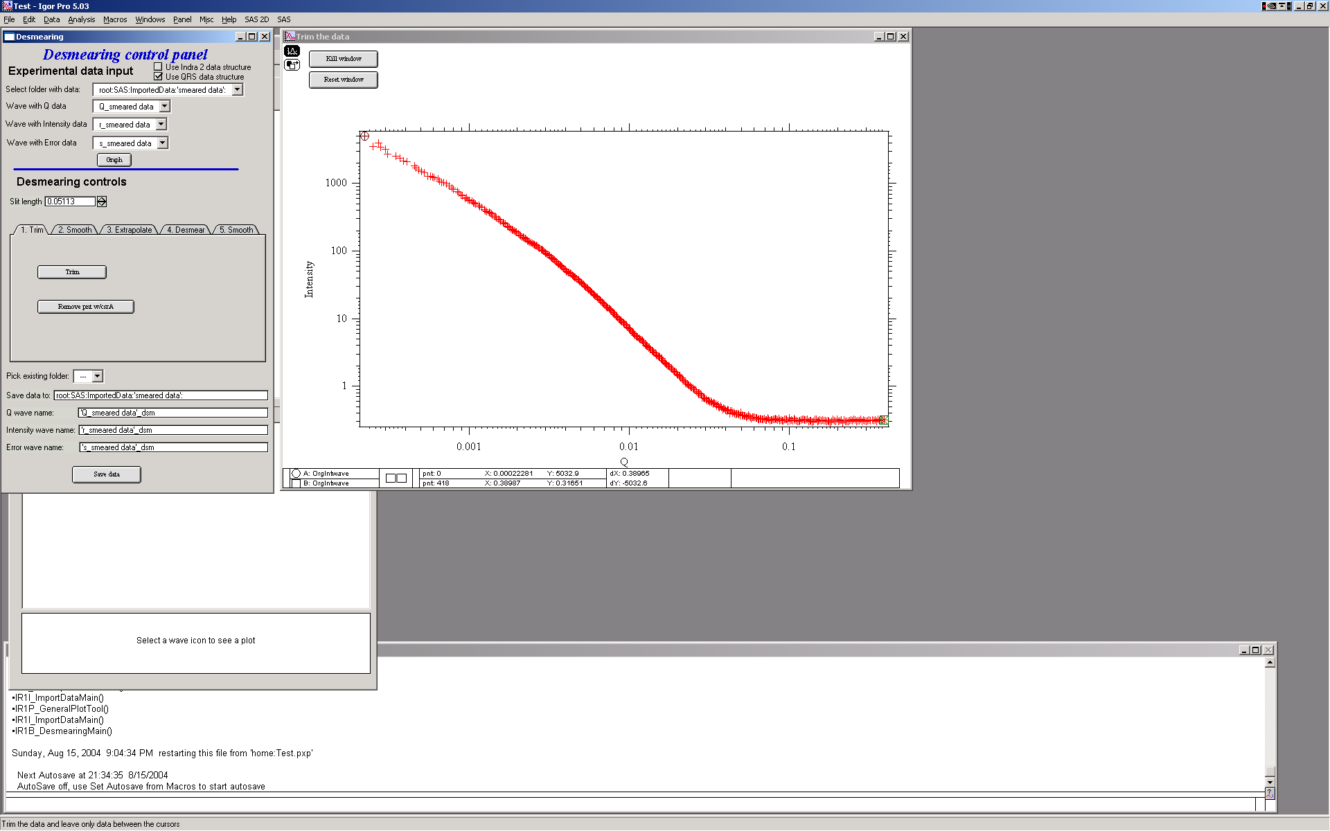
1. First step – trim usable data – small and high Q data… Use cursors to select data range. And then push button “Trim”. You can also remove any spurious point with the other button and cursor A (the rounded one)

2. Next step – it is possible to smooth data using spline smoothing, but only if necessary. I strongly discourage this… However, the screen is next:

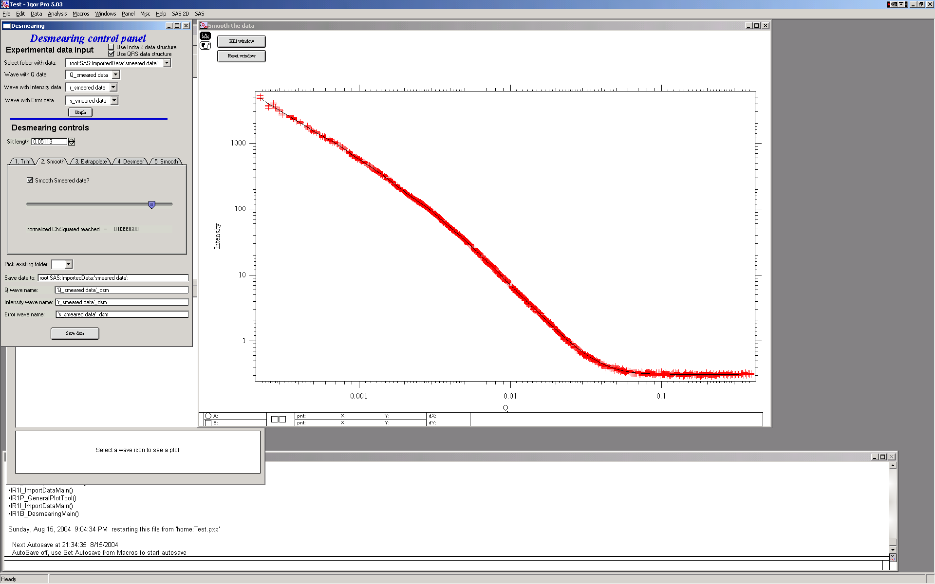
Note the slider and checkbox – the checkbox switches on the smoothing, in that case the slider appears. The slider controls the internal smoothing parameter - more to the right, more smoothing…

As I said, I discourage this, so let’s remove this in next step.

3. Extrapolating.

In order to properly desmear, I need to smear and that means I need data for at least 1 slit length BEYOND the last point. Therefore we need to extrapolate the data using one of selection of mathematical functions. Most useable one is “Power law with flat” and “powerlaw” or “flat”. These data suits best the Powerlaw with flat…

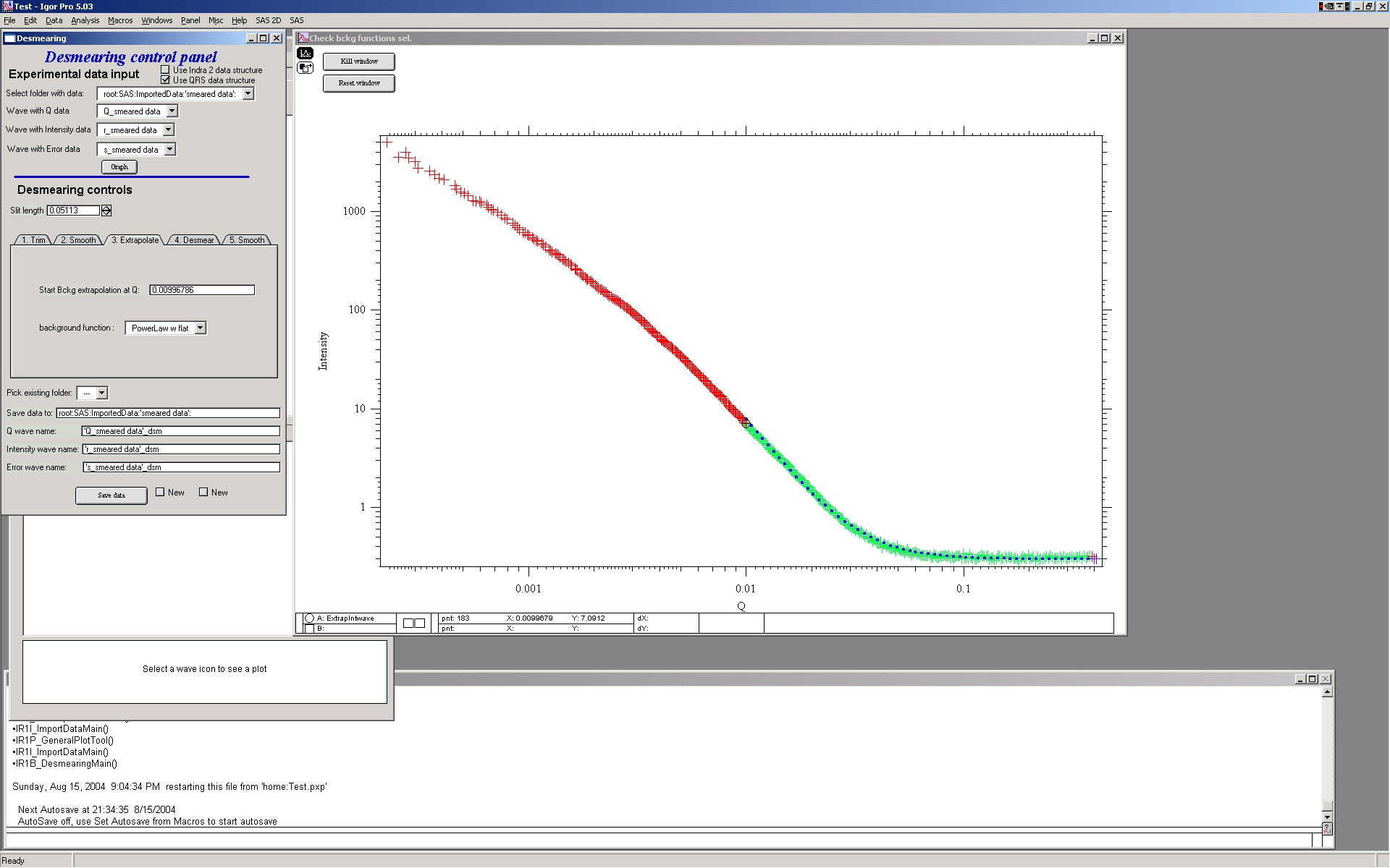
Note the colors: red are the original data, green are the original data used for evaluation of extrapolation parameters and the dotted blue line is the extrapolated data.

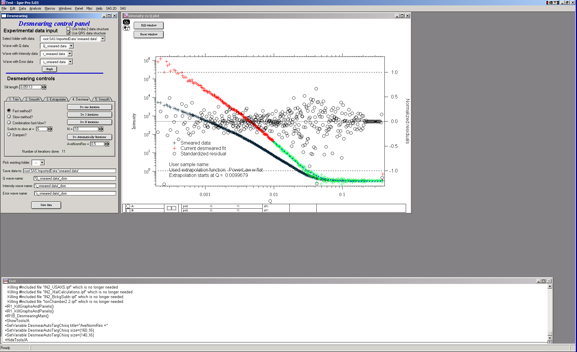
4. Desmearing

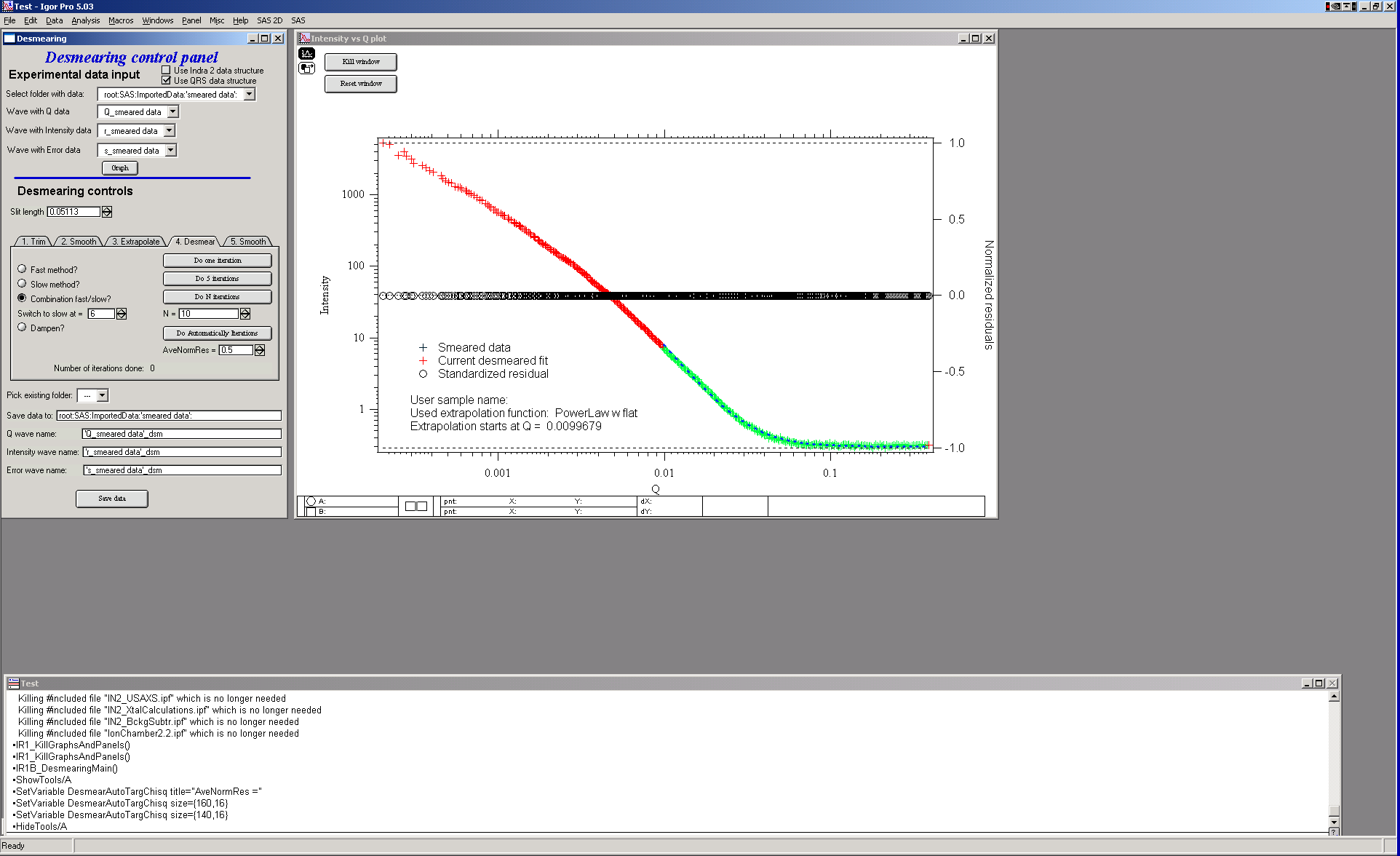
The desmearing can be done in steps – one at a time, 5 at a time, selected number of iterations at once (when you already know how many iterations are going to be needed), automatically (iterates until average normalized residual < preset value) or any combination. Also, there are two modes of conversion for Lake method: aka “slow” and “fast”. The fast method is overall the best method to use, the “slow” method iterates much slower and can result in negative number for intensity.. Combination methods – “Combination”, and “Dampen” attempt to use “fast” method (as main) and reduce formation of noise characteristic for this method. In both cases normalized residual for each data point is during each iteration compared. For combination method, if the data point is already estimated to within the user selected precision of input data (normalized residual < User input value) the point is further dersmeared by “slow” method. For dampened method, if the point is estimated to normalized residual < 0.5 it is not desmeared anymore at all…

This should reduce some of the noise created at high-q data during larger number of iterations while keeping the fast convergence of the “fast” method.

Let’s select the “Fast nethod” here, for simplicity.

Do one iteration:

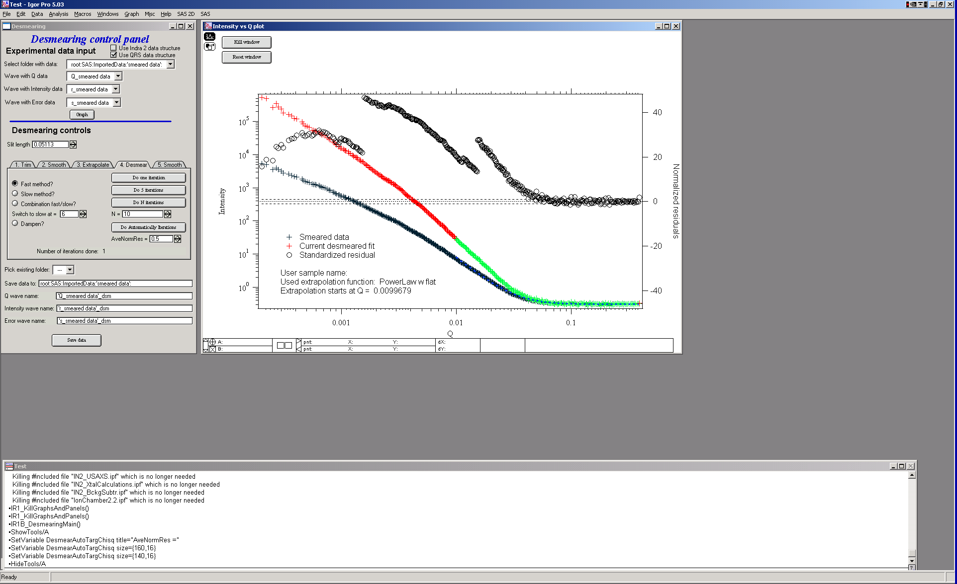
Explanation: Red/green data are current desmeared data (see above about extrapolation). Crosses are original data and circles are normalized residuals.

Desmearing should continue until the plot of the residuals becomes featureless with scatter distributed randomly about z=0 (where z is the standardized residual). Convergence is achieved when the residuals do not readjust to a significant extent between consecutive desmearing iterations. Acceptable convergence is always at the judgement of the person doing the desmearing.

For many data sets, 10-20 iterations are sufficient. Other data sets (those with more structure in the scattering curve) may require as many as 50 iterations or more to satisfy the convergence criteria of the user. For this example data set, this is about where one may end – 10 iterations and most of the circles are within +/- 1. There are some points at low Q which may need more iterations, due to the use of the combination method. (The fast method would have resolved this with fewer iterations.)

5. Final smoothing

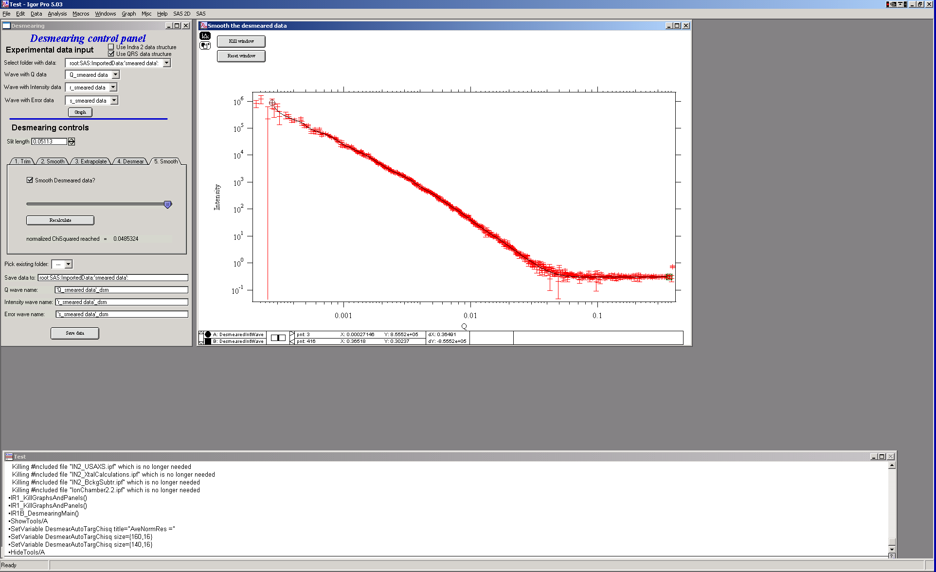
Here one can smooth data… This is probably a better place to smooth, if necessary at all.

6. Save data

Use the bottom part of the GUI panel to save data in folder of your choice. The folder, if it does not exist will be created.