Size Distribution
There are three methods to computer a size distribution from the measured SAS data:
Following is description of tool use and controls:
Basic description of methods
Maximum entropy method
Maximum entropy (MaxEnt) and regularization (maximizes smoothness) are two separate methods for obtaining size distributions from small-angle scattering data. Yet, we describe them together here since they share many common components. Both are versions of a constrained optimization of parameters which solve the scattering equation.
The difference in these two methods is in the applied constraint and it is this constraint which most heavily influences the differences between the two methods in the form of the result.
The maximum entropy method was developed by Jennifer Potton et al., and supplied in the code package MAXE.FOR. Pete Jemian (jemian@anl.gov) has had his hands all over this code and in a few places, made some rather significant additions, resulting in the code package sizes.c. Most significant is the addition of the regularization method which is likely to succeed an finding a solution in many cases when the MaxEnt method fails to converge upon a solution. Please contact him with any questions regarding the implementation of these methods. (Point of fact, both are actually regularization methods.)
J.A. Potton, G.J. Daniell, and B.D. Rainford; Inst Phys Conf Ser, #81, Chap. 3, (1986) 81-86
—J Appl Cryst, 21 (1988) 663-668
— J Appl Cryst, 21 (1988) 891-897.
J. Skilling and R.K. Bryan; Mon Not R Astr Soc, 211 (1984) 111-124.
Ian D. Culverwell and G.P. Clarke; Inst Phys Conf Ser, #81, Chap. 3 (1986) 87-96.
Literature citation for Maximum Entropy code in Irena macros bvy Pete Jemian
Pete R. Jemian, Julia R. Weertman, Gabrielle G. Long, and Richard D. Spal; Characterization of 9Cr-1MoVNb Steel by Anomalous Small-Angle X-ray Scattering, Acta Metall Mater 39 (1991) 2477-2487.
Here \(N_p(r)\) is described as a histogram size distribution where a fixed number of bins are defined over a given range of diameter with either constant diameter bins or constant proportional diameter bins. Solution of the histogram size distribution to the scattering equation 9.1 above is obtained by fitting the scattering calculated from trial distributions to the measured data and then revising the amplitudes of the trial histogram distribution based upon the applied constraints. The trial histogram size distribution is not forced to adhere to a particular functional form, such as Gaussian or log-normal. However, in the current formulation, all sizes of the scatterer are expected to have the same scattering contrast and morphology (shape, degree of interaction, aspect ratio, orientation, etc.).
In both MaxEnt and regularization methods, the measured data must be represented by the calculated data so that the goodness of fit criteria (sum of squared standardized residuals) is close to the number of measured data points used in the analysis, subject to an additional constraint. This imposes a high standard for the reported errors on the scattering intensity. The reported errors are expected to be estimates which are comparable to one standard deviation of the true intensity and that the difference between the measured intensity and the true intensity is within one standard deviation of 67% of the time and randomly distributed such that a summation over these differences has zero mean and unit RMS. If these conditions are not met, it is likely that artifacts in the derived size distribution will result. Often it is necessary to scale the reported errors by a factor to achieve converge of the MaxEnt method.
As a point of fact, both MaxEnt and regularization are regularized methods of solution to the scattering equation above. They both seek solutions of the functional, Ξ,
where \(\chi^2\) describes the goodness of fit, S is the applied constraint, and \(\alpha\) is a Lagrange multiplier used to ensure that the solution fits the measured data to some extent.
For MaxEnt, the additional constraint is that the configurational entropy of the size distribution must be maximized. Rather than be bothered by what this means when compared with the thermodynamic entropy, you are asked to consider that this constraint enforces the principle that all histograms in the size distribution must have a positive amplitude. To make the calculation of the entropy, an additional reference level must be defined. Typically, this reference level (a.k.a., Sky Background, starting guess, a priori information) is about 0.01 of the maximum level of the final size distribution. One does not need to fine-tune this parameter and should never be concerned with adjustments less than one order of magnitude. Too high and this parameter will cause the solution to have upward tails at both low and high ends of the distribution. Too low and additional scatter will appear in the distribution. The MaxEnt constraint imposes no correlation on the amplitudes of adjacent bins in the calculated histogram size distribution.
Regularization method
The regularization method implemented here maximizes the smoothness of the calculated histogram size distribution by minimizing the sum of the squared curvature deviations. The particular mathematics used here do not prevent the use of negative values for the amplitudes of the histogram size distribution and this is a noted behavior which must be considered to avoid. Often, it is possible to avoid the negative bins in the size distribution by adjusting the fitting range, the bins in the histogram size distribution, or the background.
NOTE: since version 1.50 I modified the code to provide ONLY positive solutions. It is heavy-handed code change and likely not really mathematically correct. It may change a bit in the future.
Total non-negative least square method
This is implementation of the “Interior point method for totally nonnegative least square method”. I have found reference and method description for this method on line: Michael Merrit and Yin Zhang, Technical report TR04-08, Department of Computational and Applied Mathematics, Rice University, Houston, Texas, 77005, USA. This publication was from May 2004, I have found it on the web posted in December 2004, http://www.caam.rice.edu/caam/trs/2004/TR04-08.pdf
Basically, this is very interesting method, in which one starts with reliably positive solution, calculates gradients using least square method to better solution and makes step towards this solution. The size of the step is limited in such manner, that the solution (histogram bin content) cannot be made negative. If the step would make it negative, the size of the step is limited in such manner, that the non-negativity is guaranteed.
The problem of this method is, that there does not seem to be any simple way of incorporating errors in the calculation. Generic method which was suggested to me resulted in instability of the code. So, contrary to MaxEnt method (which inherently uses errors), in this method the errors are used only to identify sufficiently good solution.
Also this method seems to have major problem with the poor conditioning of the SAS problem – natural log-q and log-I behavior of the SAS data. Therefore, it basically requires, that fitting is done in different “weighing” of the data – for example I*Q4 vs Q etc…
Uncertainties - since version 2.50 I have added code, which can generate uncertainties, by running multiple fits to data modified by adding Gaussian noise scaled to have standard deviation equal to the data uncertainties.
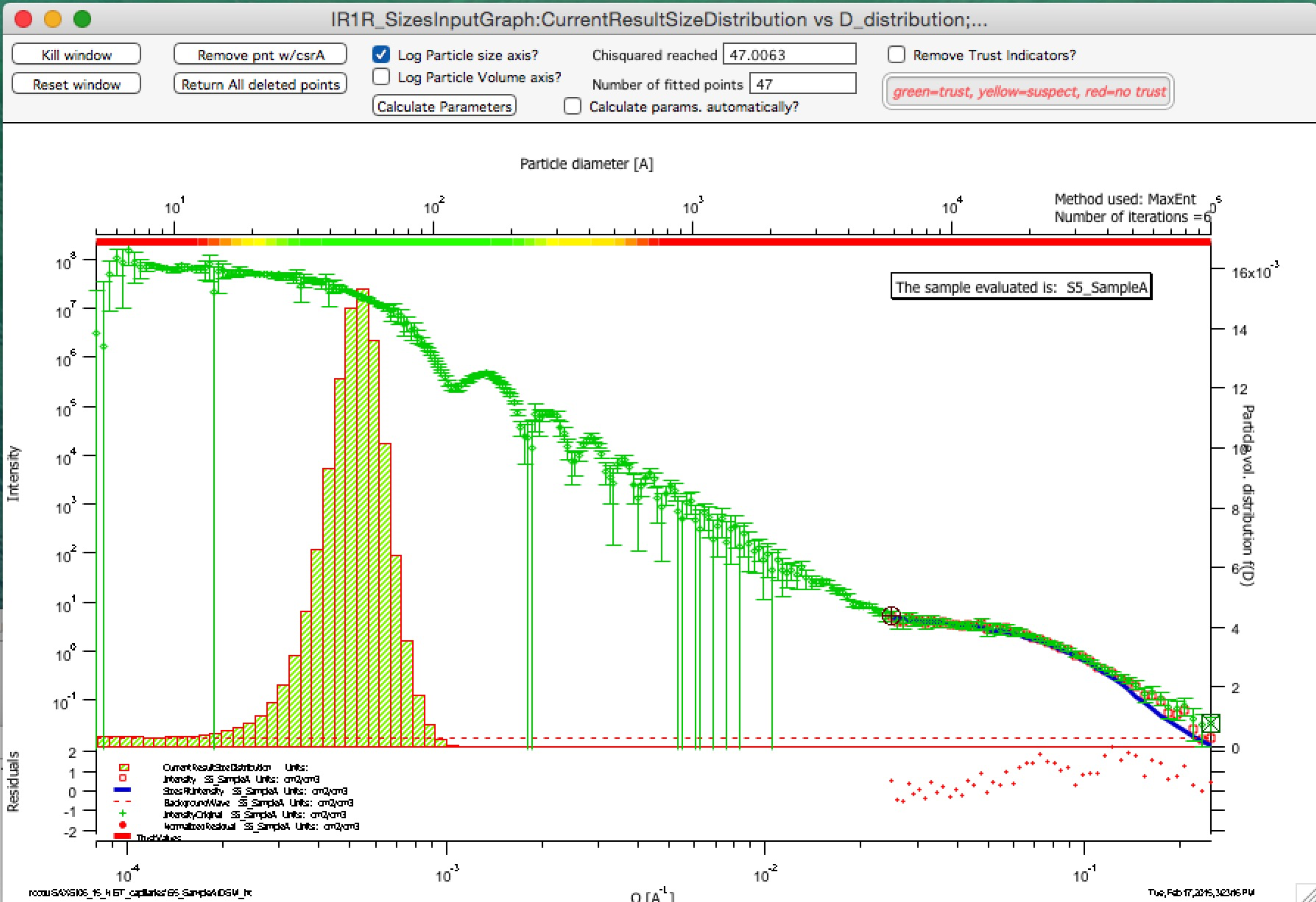
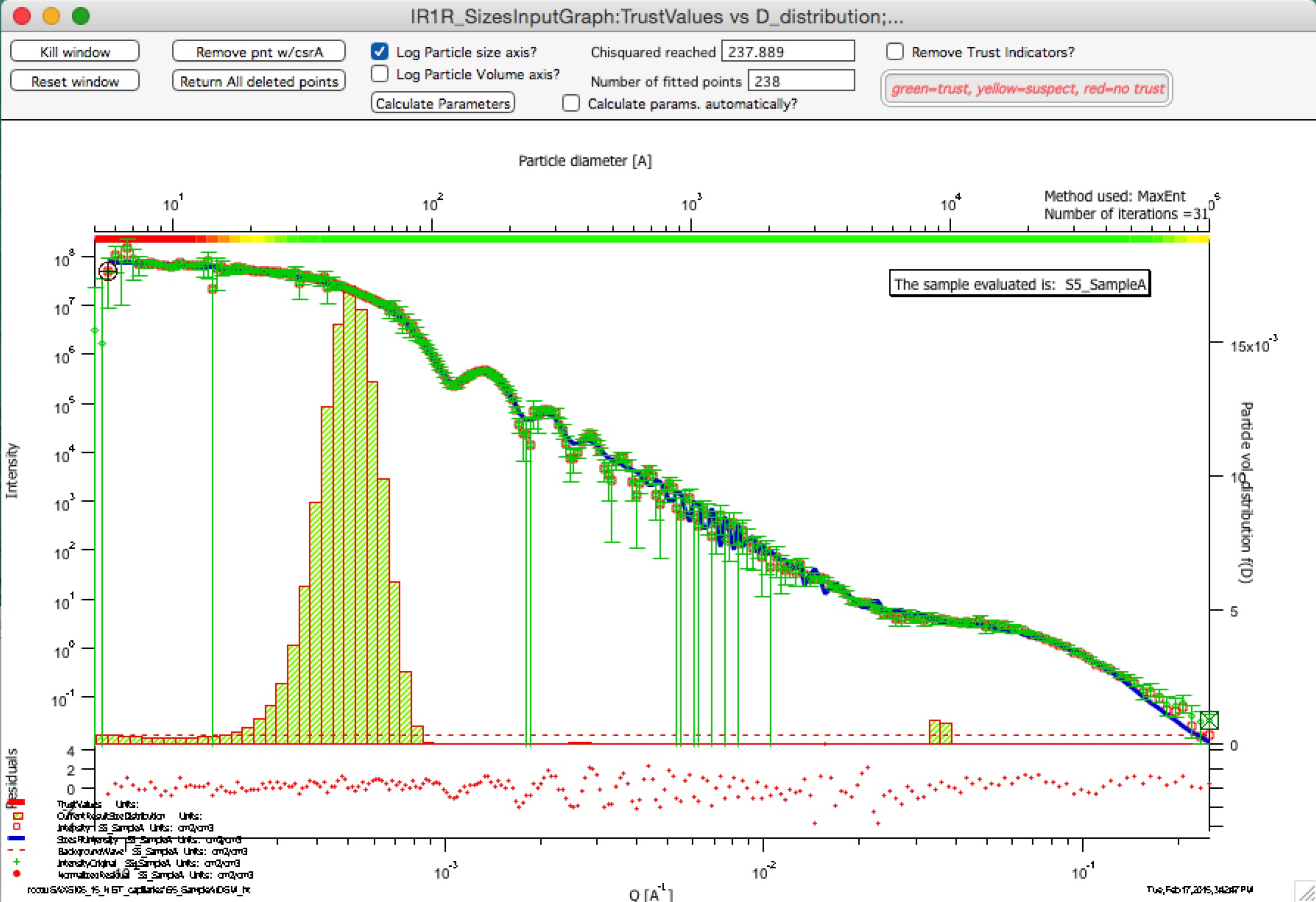
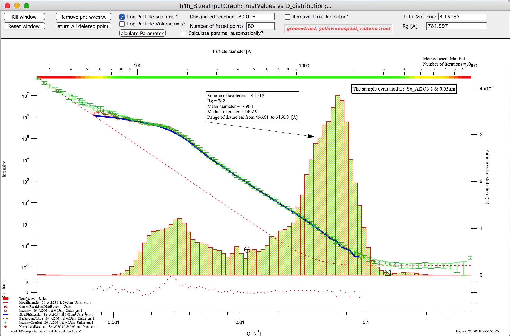
Trust regions – in version 2.57 I have added color indications about which sizes in the resulting size distribution can be trusted and which are uncertain. These calculations are pretty simplistic for now – based on Qmin and Qmax used for fitting, one can convert these to sizes (using d ~ 2*pi/Q). Only sizes of particles, which are within the measured range of Qs can be really trusted. Since SAXS sees also “outside” the fitted range to some degree, with less trust one can expect slightly larger or smaller particles to be characterized approximately, and as one gets far from the fitted Q range with sizes, trust in the results should be very small. This is indicated on the trust indicator – green center part shows trusted range, yellow transition suspect range, and red ranges are simply untrustworthy. The tool will produce something, but with no bounds by data, this will be pure speculation with no real value. This color bar can be removed using checkbox at the top bar of the graph.
Compare following two graphs, in which the Q fitting setting is vastly different:
Next is description of how to use the tool.
Use of Size Distribution
This manual is updated for Size distribution tool version in Irena 2.67 and higher, for older versions see prior versions of manual. Test Igor experiment is available on following location:
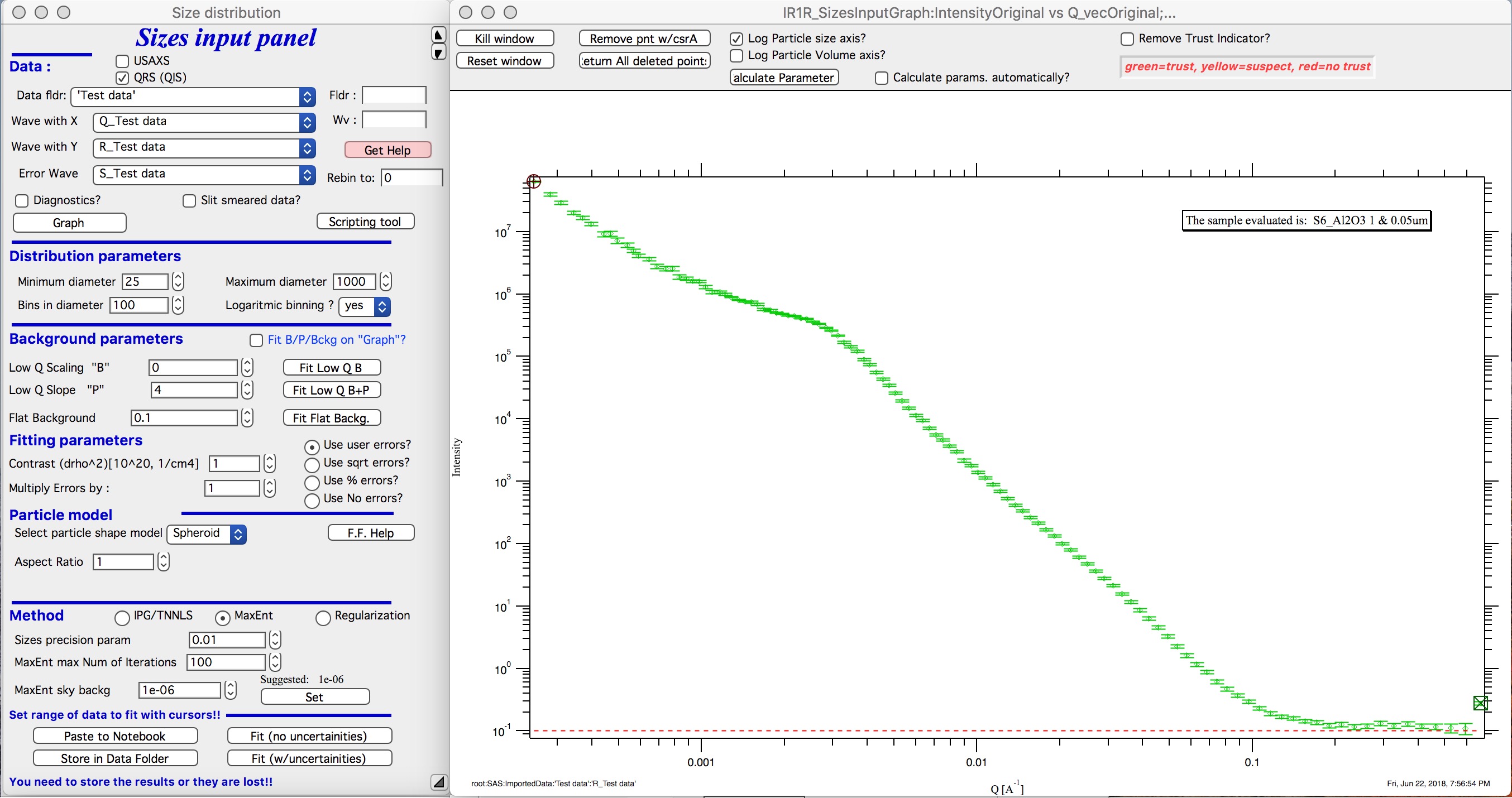
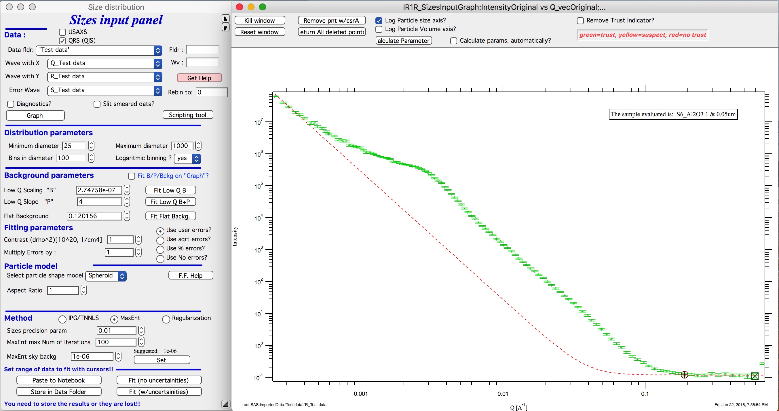
This program uses one complex interface – a complex graph and panel for data input and manipulation. To start, select “Size distribution” from “SAS” menu…
On the panel, which gets created, starting from top are standard data selection tools. This package can also be scripted by scripting tool
- select the “Use QRS checkbox” (assuming you are using QRS named data as explained above).
- Select data folder with data (see image below)
- Select wave with Q vector, other should be selected automatically (if not select right waves). Note, that it is now not necessary to input error wave. See below…
- “Graph”
New graph gets created.
Leave the “Slit smeared data” unchecked, unless you have slit smeared data. If using the Indra data structure (USAXS data), slit smearing is selected properly when needed and settings should not have to be changed. If the data would be from different instrument and would be slit smeared, then select slit smearing and insert slit length. I expect this case to be highly unlikely…
Next we need to setup fitting parameters.
Distribution parameters:
Minimum diameter & Maximum diameter – both are in A. These are limits of fitted distribution. Set minimum to 25 and maximum to 10000 for the test data (these data are included with Irena distribution as Test data.dat).
Bins in diameter – into how many bins you want to divide the range of diameters. 100 is a good number – more points may be slow on slower computers.
Logarithmic binning – if yes, the bins are binned logarithmically – i.e., the bins at small sizes are smaller and at large sizes are larger. This is useful setting when wide ranges of scatterer sizes is measured using wide q range (USAXS/SAXS type) instruments. If no is selected here, the bins are all same width. Leave in yes for now…
Background parameters
Current version of Size Distribution can use two functions for background and often both may be needed - but not always. Note, that until 2018 release of Irena v2.66 this tool had only Flat Background. The background is subtracted from the data before fitting and in the graphs it is displayed as red dashed line. The purpose of next few paragraphs is to get this dashed line to match physically meaningful, defendable, estimate fo scattering which needs to be subtracted from the data.
Note, that use with slit smeared data is bit complicated here, background is not slit smeared by the code and so it may be bit challenge to use.
- Flat background. This is common for most SAXS and especially SANS instruments, that some amount of flat background is present in data. This is typically at high-q, often it may be solvent scattering and similar origin. While more complex background are possible, this tool assumes flat (fixed value) background independent of Q.
- Low-q power law slope. This is also quite common - data exhibit low-q power law slope. This could be grain boundaries, powder surfaces, scratches on the sample surfaces, large aggregates etc. There is huge number of possibilities for sources of power law scattering at low-q and if not subtracted, this impact resulting size distributions.
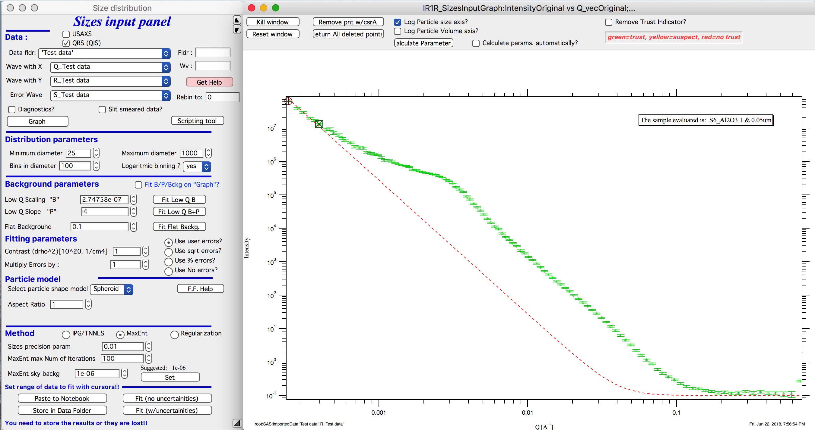
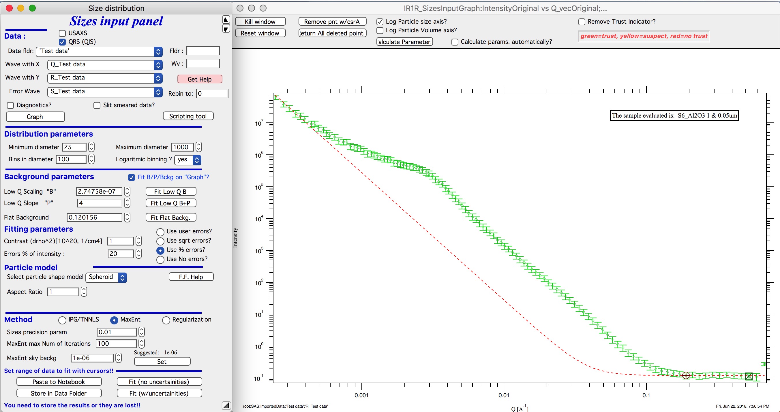
First the low-q power law slope
Select first five points with cursors. We have two options - two buttons :
- “Fit Low Q B” : this fits only power law scaling factor (B in Unified fit) and keeps existing power law slope itself (P from Unified fit). Default P is 4 = Porod’s slope. This is often good assumption in case of scratches or powder grain surfaces. In this case (these are powders) keeping P=4 is correct choice. When the proper Q range is selected (possibly proper P is manually set) push button “Fit Low Q B”
- “Fit Low Q B+P” : this fits both power law scaling factor (B in Unified fit) and power law slope itself (P from Unified fit). This is often good assumption in case of second population of scatterers with wide size distribution. Do not use this to fit aggregates as this tool is missing RgCo parameter which would be needed to terminate the scattering from aggregates at the size of primary particles. This Size Distribution tool is really not suitable for fitting aggregated systems anyway.
Below is result of fit at low-q using fitting of only B parameter with P=4.
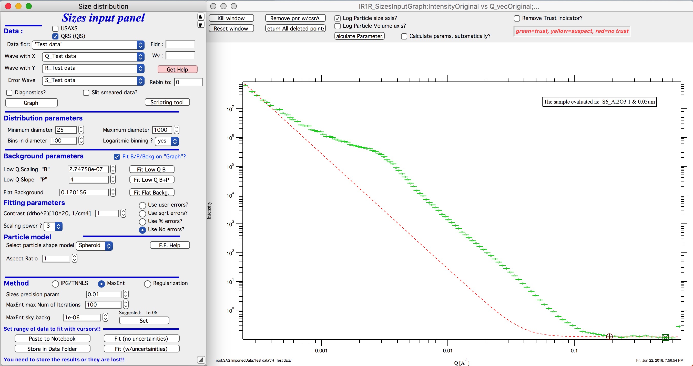
Next is fitting of Flat background.
As you can see, at high-q the red dashed line nearly touches the data (ignore the last point which is artifact). It is nearly correct (by accident here). Users can either manually change the background (type in value or use arrows on the right hand side of the set variable field). Or we can fit this. Set cursors between points 100 and 110 - this is area where flat background dominates.
- “Fit Flat backg.” : this fits flat background assumption between the cursors.
Here is result of the fitting:
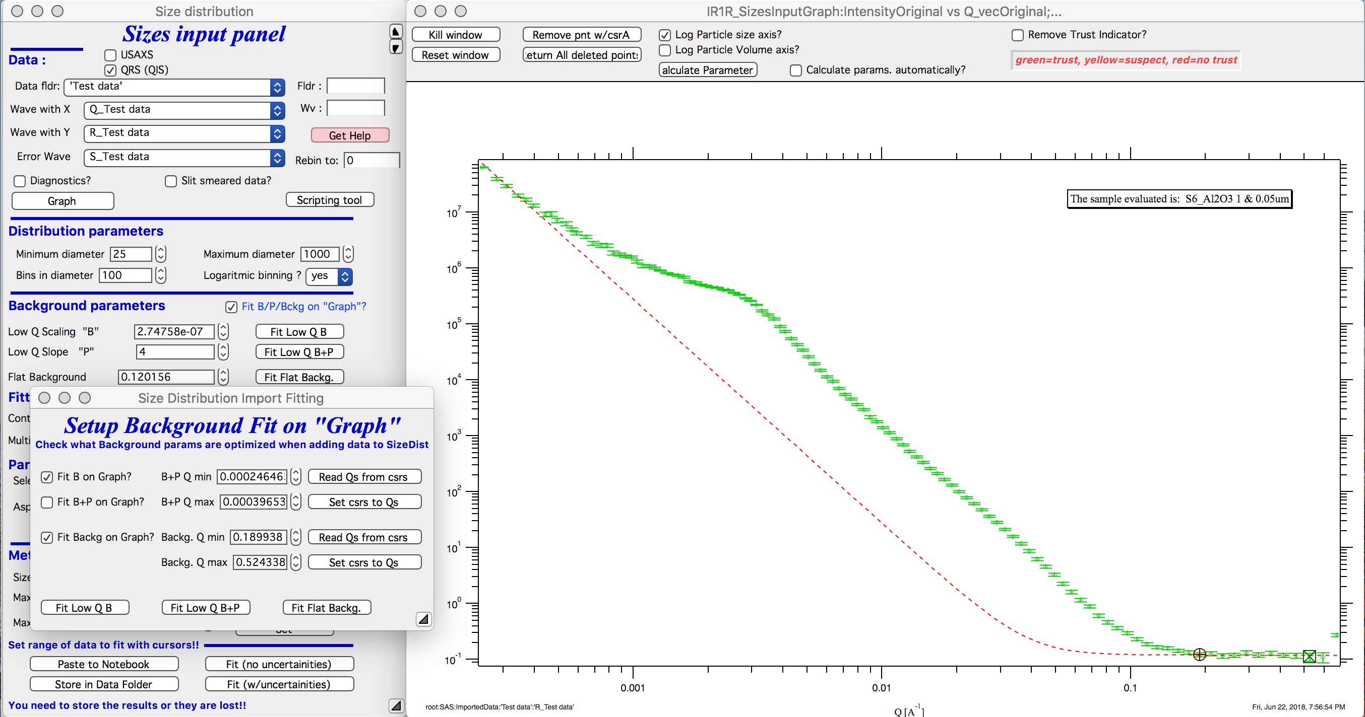
Optimizing of these “Background parameters” on data import
If one wants to analyze large number of data sets, especially using scripting tool, manual changes to these three parameters are highly inconvenient. Therefore there is add on tool in this part which allows optimization of these parameters automatically, when user pushes button “Graph”. To achieve this we need to setup what will be done and in what Q ranges.
Checkbox : Fit B/P/Bckg on “Graph”
When selected a new panel appears:
Select if you want to fit only B or P+B using “Fit B on Graph?” or “Fit B+P on Graph?”. Here we will use just the B, so check checkbox “Fit B on Graph?”. Set cursors on points 0 to 5 and push button “Read Qs from csrs” next to the two top Q vales. You can also type in Q values manually in these fields.
Check “Fit Backg on Graph?” and select high-q data points 100 - 110 with cursors and push button “Read Qs from csrs” next to the two bottom Q vales. You can also type in Q values manually in these fields.
You can test the fits using the button for “Fit …” - they do same as in the main graph. You can test settings of the cursors for the different fits.
Now, when new data are added in the tool using button “Graph” both B and Background will be optimized in the Q ranges selected. If you do not want to do this, simply uncheck the Fit B/P/Bckg on “Graph” checkbox and it will also close this secondary panel. Note: you can close this panel if not needed anymore, to reopen simply uncheck and check the checkbox Fit B/P/Bckg on “Graph” on the main panel.
Fitting parameters
Contrast (\(\left| \Delta\varrho \right|^{2}\)) – if this is properly inserted, the data are calibrated… Leave to 1 since the contrast is not known.
Error handling
There are four ways to handle now errors in this tool. The method is selected by four checkboxes lined vertically next to the “Background and Contrast” fields…
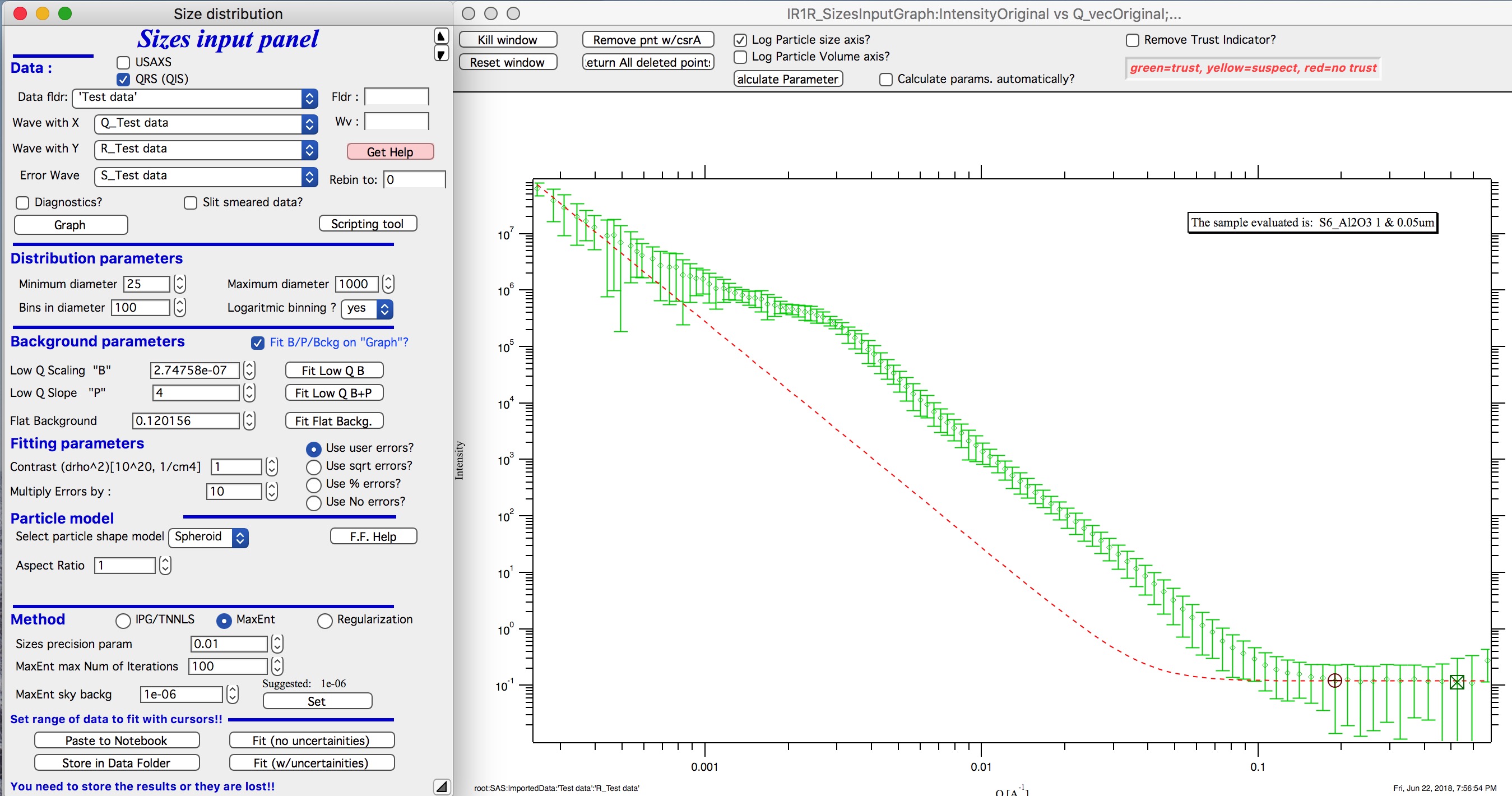
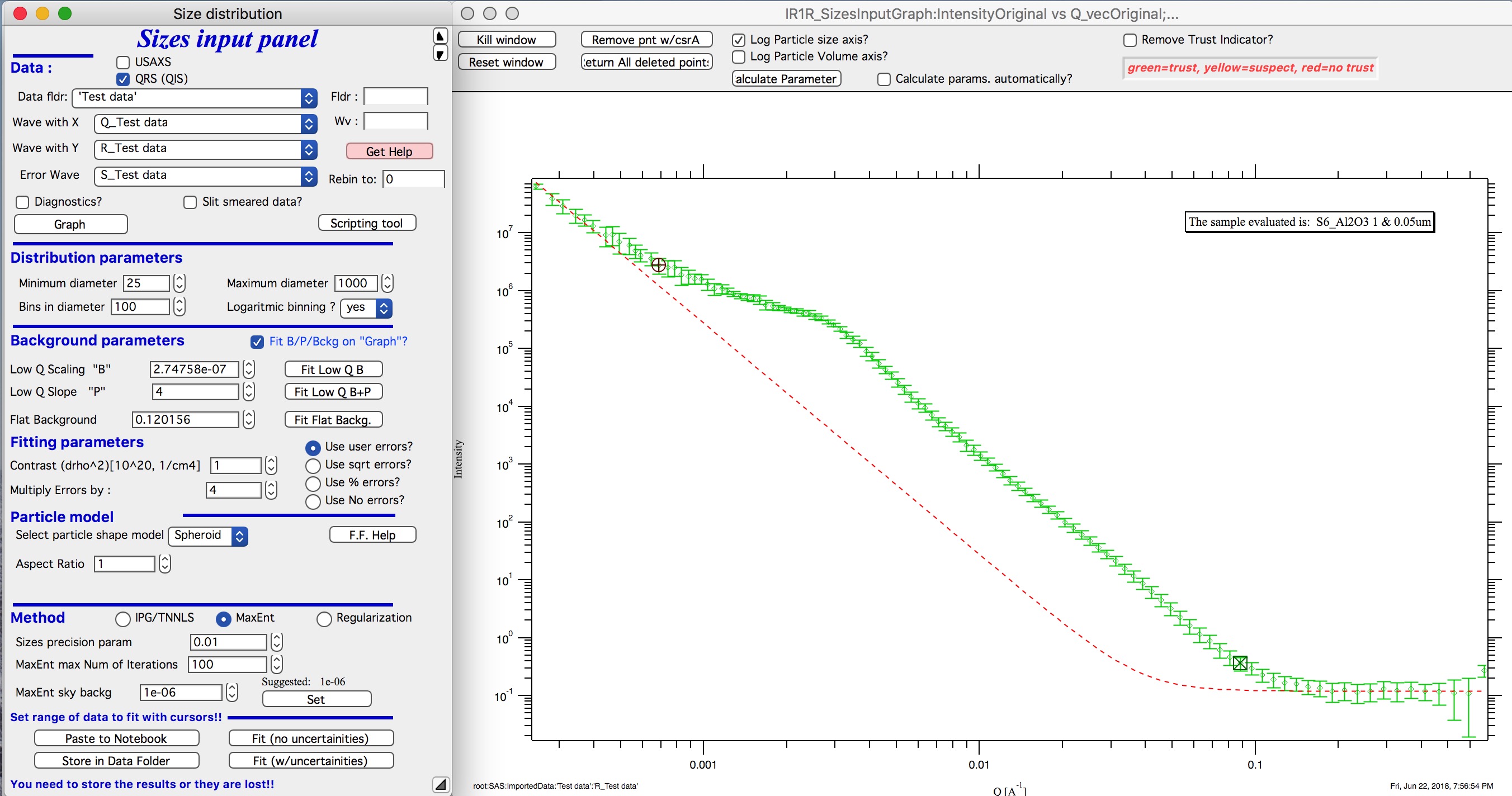
- “Use user errors” use error input as wave. In this case the field: “Multiply errors by”is available and errors can be scaled as needed. Start with high multiplier and reduce as necessary to reach solution, which is both close to the data but not too noisy.
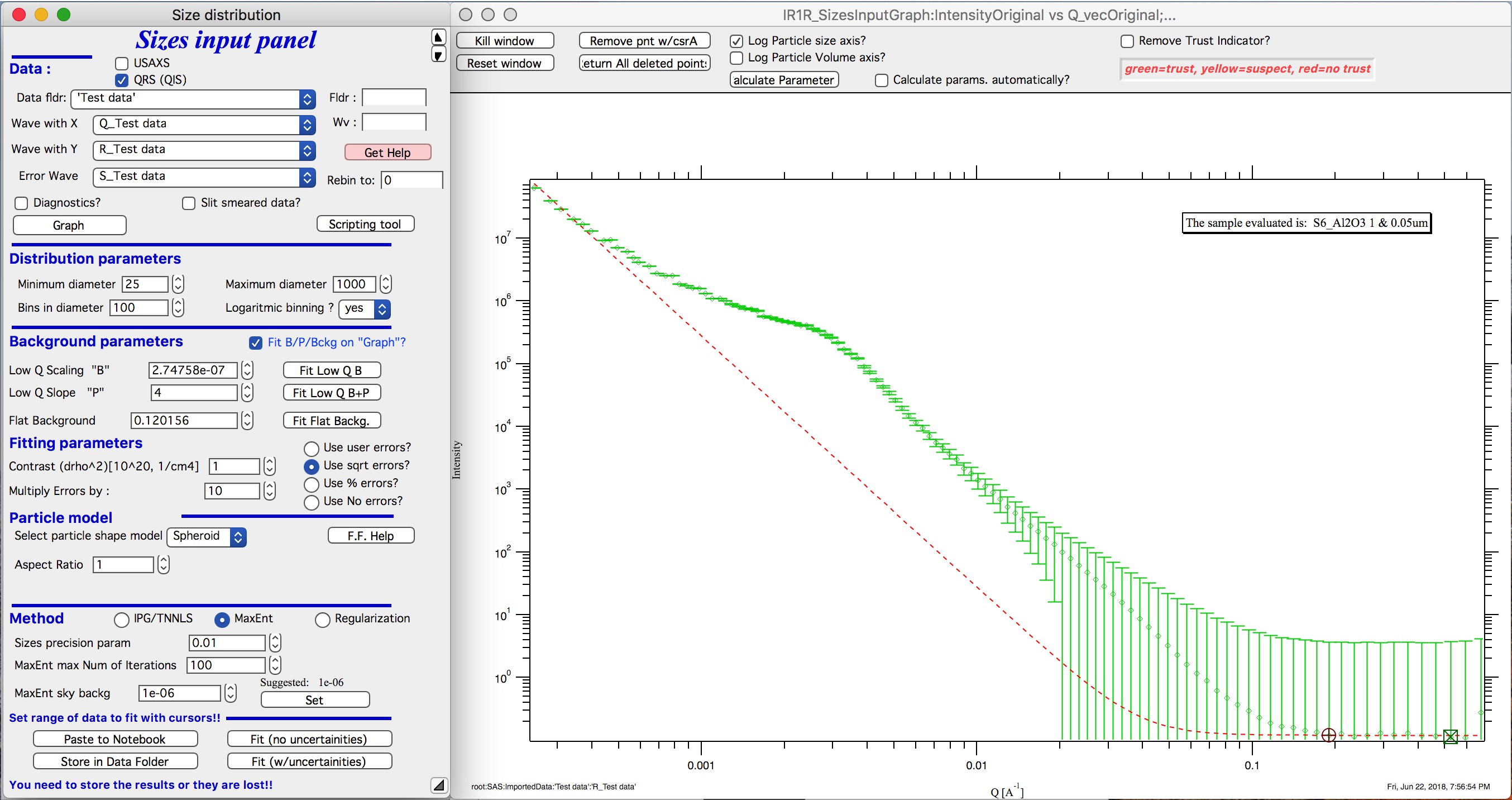
- “Use sqrt errors” – will create errors equal to square root of intensity (standard Poisson error estimate). You can multiply these errors by error multiplier. Errors are smoothed.
- “Use % errors” – will create errors equal to n% of intensity. Field where to input the n appears. Errors are smoothed.
- “Use No errors” – use no errors – the weight of all points is the same. This is unlikely to be correct, but this case allows to use fitting in “scaled” space – Intensity * Qm vs Q, where m = 0 to 4. This helps to mathematically better condition problem (similarly to using errors) and can yield sometimes good solution. NOTE : at this time you cannot use this method (no errors) with MaxEnt or Regularization, this is useful ONLY for IPG/TNNLS method.
Comments:
MaxEnt works best with user errors or % errors. Good User errors are preferred.
IPG/TNNLS seems to work best with no errors and m = 2 - 4. Reason is unclear.
The errors displayed in the graph will change as different methods are selected:
User errors, multiplied by 10:
SQRT errors, multiplied by 10:
% errors, used 20%:
No errors, selected to use I*Q3 vs Q “space” for fitting:
Particle shape
Particle shape model – the tool uses the smaller selection of form factors as Modeling tool. Adding more form factors makes no sense here, with enough size distribution everything looks like a sphere.
Aspect ratio – anything, 1 is for sphere.
Methods
The default method is Maximum Entropy.
Size precision parameter is internal number which should not be changed too much. Most users should be happy with default. Smaller the number, more precisely MaxEnt needs to match the chi squared…
MaxEnt max number of iterations – unlike Regularization, which has limit on number of iterations, MaxEnt can go infinitely. Therefore maximum number of iterations need to be enforced.
MaxEnt Sky Background. While this is relatively complicated number internally, note the suggestion next to it. Suggested value is 0.01 of maximum of the resulting volume distribution. The suggested value will be either green or red, depending if the value in the box is reasonable. Accept the suggestion and you will be happy.
IPG/TNNLS

Approach parameter is the step size (from maximum) which will be made in each step towards calculated ideal solution. Basically convergence speed, but too high number will cause some overshooting and oscillations. For most practical purposes seems to work fine around 0.5-0.6.
NNLS max number of iterations – limits number of iterations. Change as needed.
Scaling power – this is how Intensity will be scaled to improve the conditioning of the problem.
Regularization
Has no additional controls.
Buttons part
Fit (no uncertainties) runs the above selected method on the data, fitting the date between cursors after subtracting the background model (dashed red line).
Fit (w/uncertainties) runs the above selected method on the data, fitting the date between cursors after subtracting the background model (dashed red line). But this will run 10x and for each data set it will add noise on scale of the “errors” provided by user. Than results are analyzed and average size distribution with uncertainty for each size bin is generated. This enables users estimate uncertainty for the resulting size distribution. This is uncertainty related to “statistical uncertainty” of measured intensities.
Paste to Notebook Makes notes in notebook Irena keeps for users. Users can add more material in this notebook.
Store in Data Folder Resulting size distributions and intensity vs Q fit data are stored in the folder where the data came from. This will keep generating new “generations” of results (_0, _1, _2,…), so it can become real mess if saved too many times.
Getting fit.
OK, above in “Background parameters” we have already configured that we will want to subtract underlying Porod’s scattering from low-q and flat background. We fitted the parameters and the dashed red line describes well what we want to subtract. Also, make sure the Minimum diameter is 25A and maximum diameter at least 10000.
Next, let’s select range of data using the cursors which will be fitted. Set rounded cursor on point about 13 and squared on point 92 or so. Note, that you can vary the range of fitted data between the fits.
Scale the Errors up, set scaling to 4 or so.
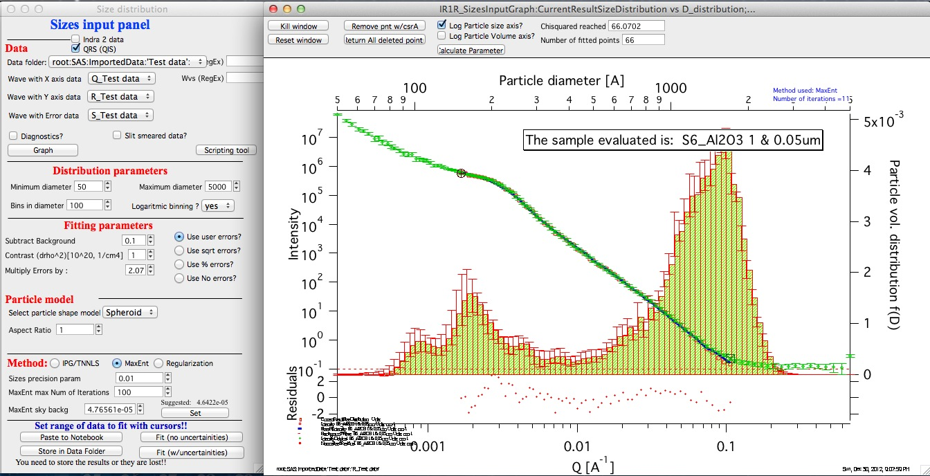
Push button “Fit (no uncertainties)”. Solution should be found as in the image below…
If the parameters are too restrictive you may get error message, that solution was not found. In such case check minimum and maximum diameter settings, check the error multiplication factor etc. Generally I suggest starting with higher range of diameters than needed and higher error multiplication factor. Then reduce as needed.
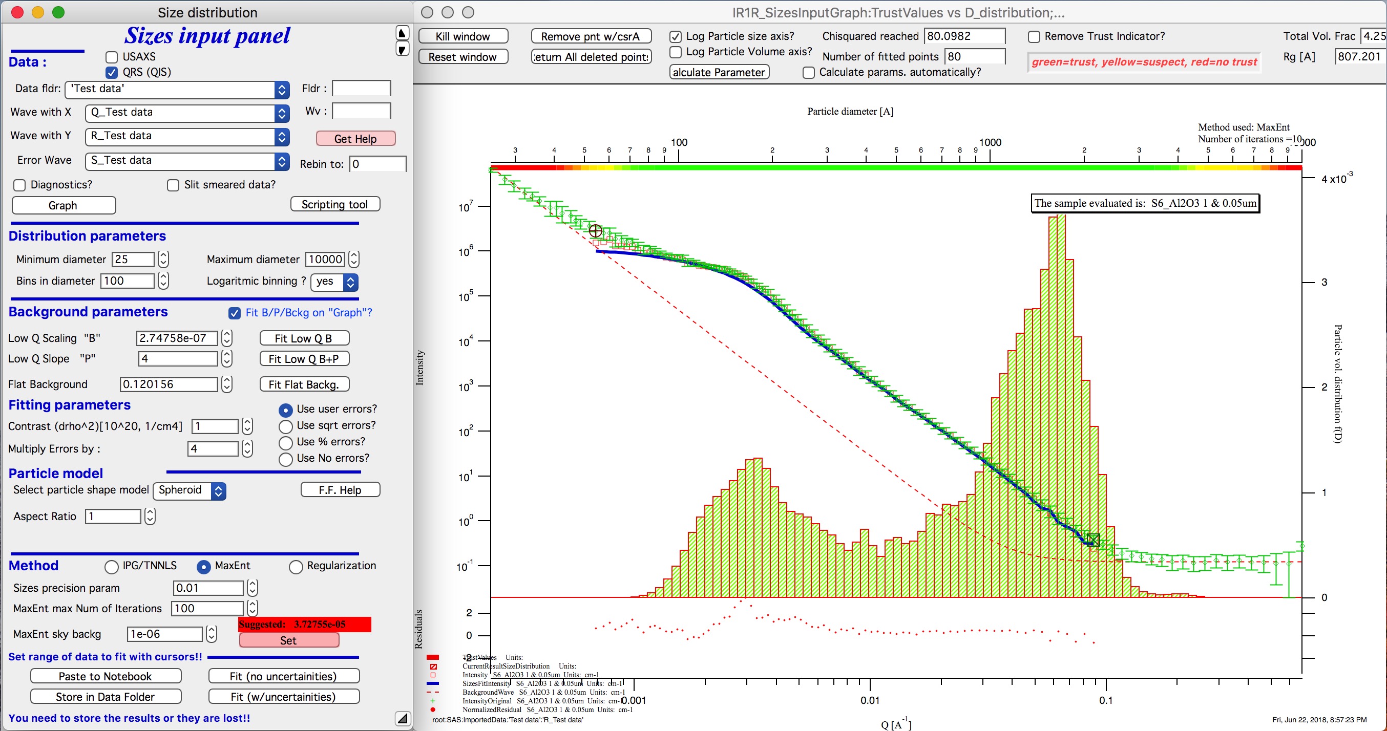
This is rough fit for the data in the graph – and for purpose of description of this graph now.
Now let’s get to explanations:
To get better results one now needs to play with the parameters. I suggest reducing multiply errors by to 3.
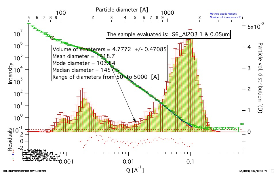
IMPORTANT: you need to fix the MaxEnt sky background when that “Suggested” red block appear, simply push the button. Running the same routine again. Following is the result:
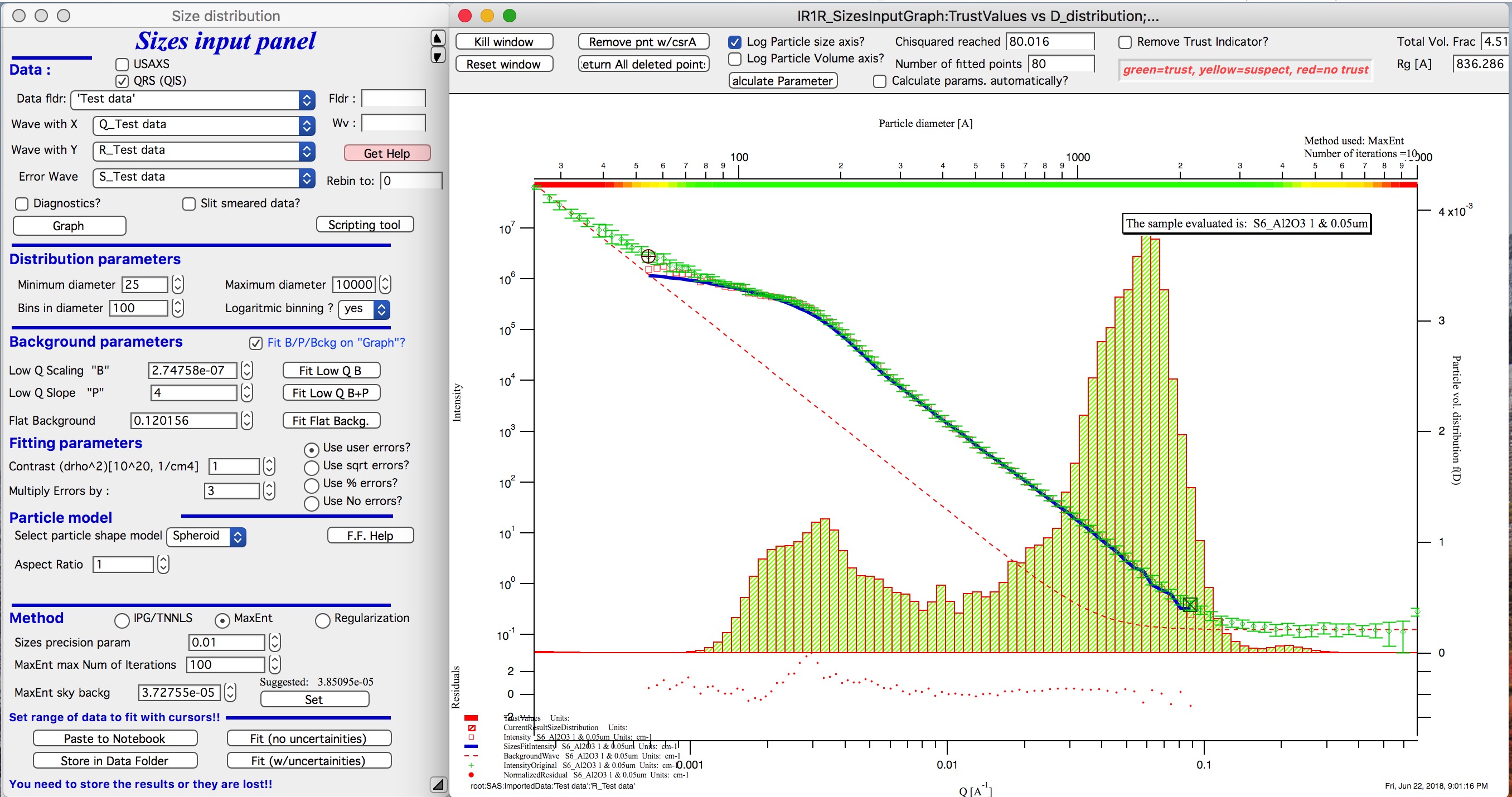
This shows, that we have bimodal distribution of scatterers. By the way, these data are from mixture of two polishing powders.
And now the IPG/TNNLS method:
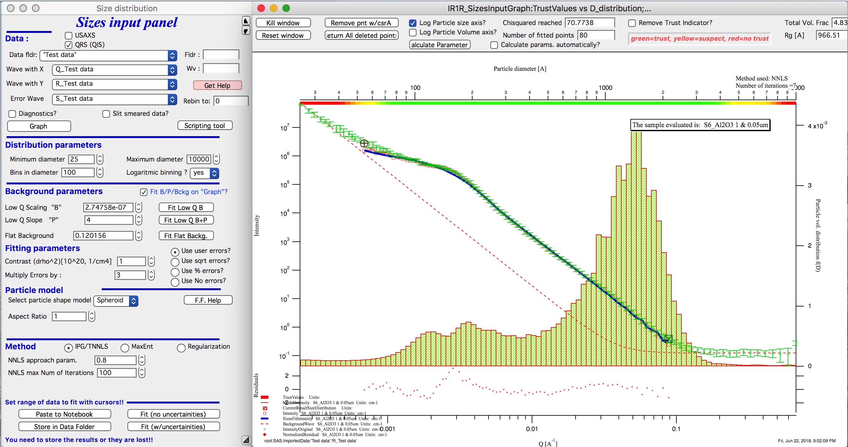
This is solution with user errors. Note, that the solution is basically very similar to MaxEnt.
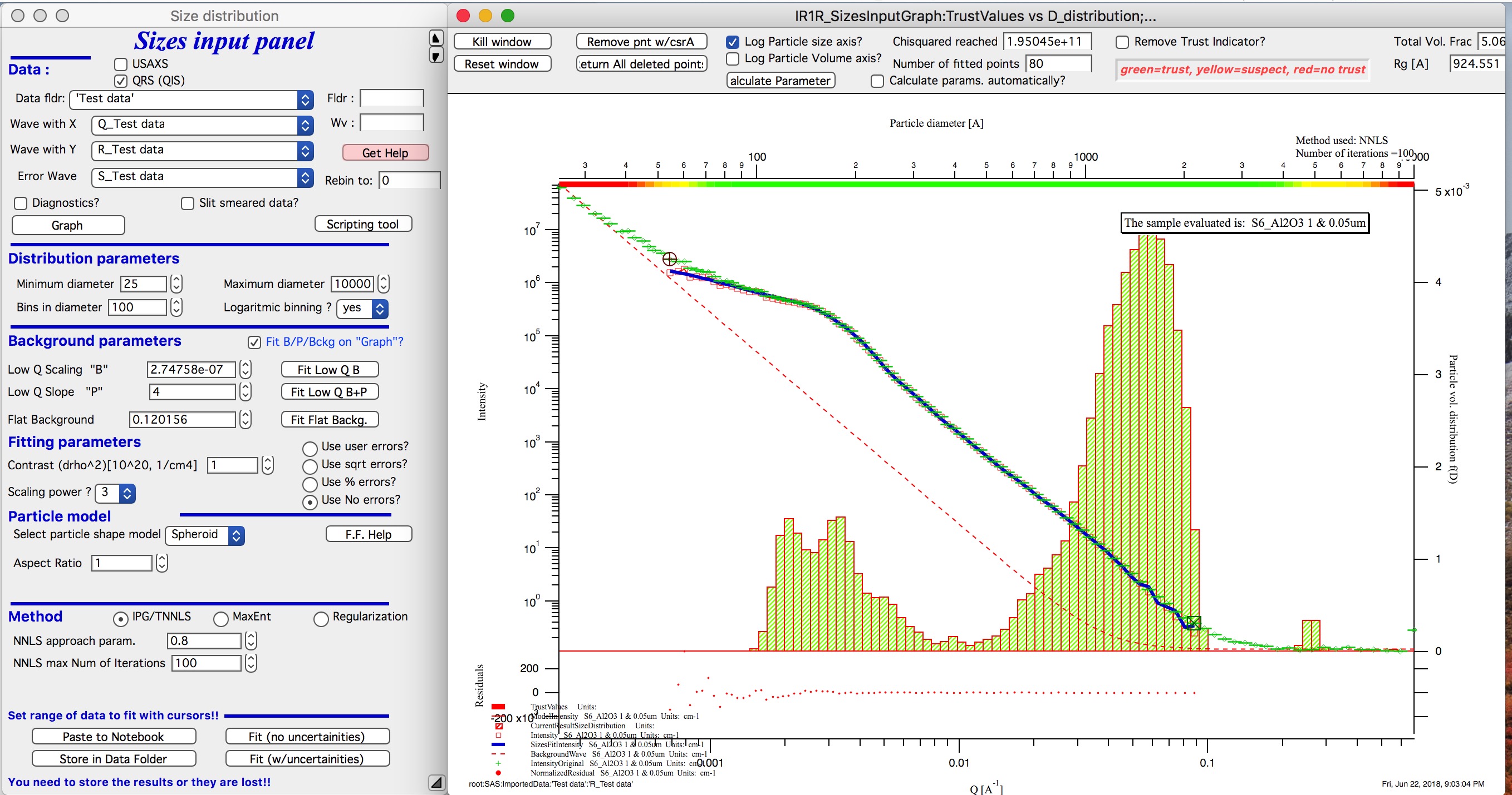
And here is solution with no errors, but scaling by Q3. Less noisy. Note, that in this case the IPG/TNNLS method is stopped by the Maximum number of iterations. Less number of iterations, less noisy solution – but may not be close to measured data…
NOTE : at this time you should not use this method (no errors) with MaxEnt or Regularization.
Saving the data copies waves with results into folder where the measured data originated. Also, it is possible to have various generations of data saved. In order to give user chance to find what each saved result is, following dialog is presented:
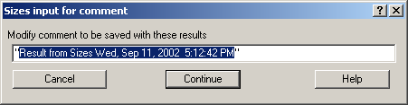
Here user can write ANYTHING, as long as it is bracketed by the QUOTES. The QUOTES are VERY important.
If user tries to start Size distribution macros in folder, where saved solution to this method exists, he/she is presented with dialog, which allows one to recover most of the parameters used for that solution.
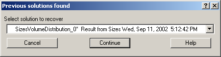
Therefore it is possible to start from where he/she left off. Also it is possible to start fresh - just hit cancel in this dialog - when parameters are left in the state they are left in after last fitting (or in default if this macro was not yet run in this experiment.
Comment: each of these waves contains WaveNote, which contains most of the details about how the particular results were obtained. The names and meaning depends a bit on method used.
Most of these parameters should have self explanatory names. This is where user can figure out what happened.
Further some parameters are also saved in the string with name “SizesParameters_0” such as MeanSizeOfDistribution.
Uncertainty analysis of Size distribution
If “Fit (w/uncertainties)” is used, 10 fits with data varied by data modified by Gaussian noise scaled to ORIGINAL uncertainties is run and statistical analysis is done on each bin. Here is example of results:
Note, that the tool can provide calculations of volume with uncertainities:
The uncertainties are exported and plotted. More support in Irena needs to be added as needed.
Graph information and controls
Graph of size distribution has number of useful bits of information:
- You can display data with log or linear axes
- You can use the trust bar or remove it
- The code automatically calculates volume fraction over all of the fitted size distribution - if the data are on absolute intensity scale and user provides correct contrast, the value here is volume fraction of the scatterers.
- Code also calculates Rg fro the system using all of the diameters.
- Using button “Calculate Parameters” one can select range of size distribution data and get Tag with useful information about that range of data.