Model description
This chapter describes the mathematical models available for scattering populations in the Modeling package. Any population can use one of the following types:
“Size distribution”“Unified level”“Surface fractal”“Mass Fractal”“Diffraction peak”
This flexibility allows modeling of complex small-angle scattering data. The Small-angle diffraction tool and the Fractals tool also use some of these models.
Size distribution
Size distribution parameters are described on the main Modeling package page. The size distribution can use any of the form factors and structure factors available in Irena. See: Form and Structure factors. For GUI details, assumptions, and distribution shapes, see: Size distribution.
Unified Fit
The Unified Fit uses the formula explained in the Unified Fit model page: Unified Fit.
Diffraction Peaks
Diffraction peak shapes are used in the Small-Angle Diffraction tool and in the Modeling package. The following formulas define the peak profile Ψ(x) for each available shape:
Gaussian Function
where σ is the Gaussian width, μ is the peak center, and M is the scaling factor.
Modified Gaussian Function
where d ≥ 1 is the exponent controlling the falloff rate.
Lorentz Function (Lorentz-squared is this function squared)
where a is the Lorentzian width.
Pseudo-Voigt Function
where x0 is the peak center, w is the FWHM, and 0 ≤ η ≤ 1 is the weight parameter. η = 0 gives a pure Gaussian; η = 1 gives a pure Lorentzian.
Pearson type VII Function
where a is proportional to the FWHM and m controls the tail falloff rate.
Gumbel Function
where β is the width and μ is the peak center.
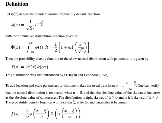
Skew normal function
Percus-Yevick S(q) and Percus-Yevick S(q) × Sphere F(q) — described in the Form factor and Structure factor PDF (accessible from the SAS menu in Igor Pro). The P-Y S(q) code is derived from the NIST SANS data analysis macros.
Surface and Mass Fractal
This model was developed for analysis of fractal systems in cement, see: https://www.nature.com/articles/nmat1871. For more details, see also: Fractal model. When possible, use the dedicated Fractals tool — it is simpler to use than configuring this population type in Modeling.
The model predicts QDv scattering (between Q-1 and Q-3) for mass or volume fractals, and Q6-Ds scattering (between Q-3 and Q-4) for surface fractals.
The full model for dΣ/dΩ as a function of Q contains four components:
dΣ/dΩ = {VOLUME FRACTAL + SINGLE GLOBULE} TERM + SURFACE FRACTAL + FLAT BACKGROUND
These components are incorporated into the full theoretical expression as follows:
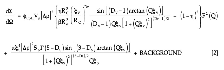
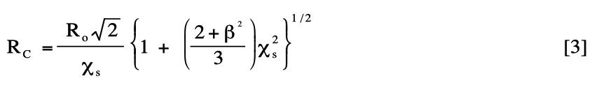
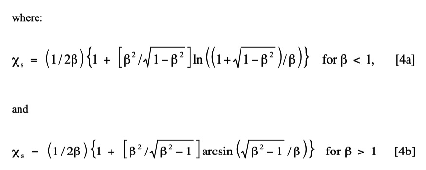
The first volume-fractal term contains ΦCSH, ξv, and the mean radius Ro and shape aspect ratio β of the building-block C-S-H gel globules in the volume-fractal phase (assumed to be spheroids). It also contains a local volume fraction η and the mean correlation-hole radius Rc — the mean nearest-neighbor separation of gel-globule centers. Rc, weighted over spheroid surface contacts, is given by:
The single-globule term arises because nearest-neighbor solid particles cannot overlap (centers cannot approach within Rc). This correlation-hole effect makes individual particles distinguishable even within an aggregated structure, at length scales of order Ro. For a spheroid of aspect ratio β, the single-globule form factor F:sup:`2`(Q) is given by:
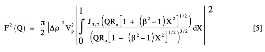
where Vp = (4βπRo/3), J:sub:`3/2`(x) is a Bessel function of order 3/2, and X is an orientational parameter integrated over all orientations of the spheroid with respect to Q. A mildly spheroidal shape avoids the pronounced Bessel function oscillations for perfect spheres (β = 1) that can perturb fits at high Q. Both mildly oblate (β = 0.5) and mildly prolate (β = 2) shapes give equivalent fits for cement systems.
The surface fractal term includes ξs, the upper limit of surface-fractal behavior, and So, the measured smooth surface area per unit sample volume. The term Γ(5 − Ds) is the mathematical gamma function.
The BACKGROUND term represents incoherent flat background scattering, usually subtracted from both data and fits for convenience.