Reduce WAXS data

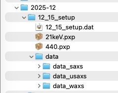
When you collect data on the USAXS instrument, data are saved in folders named using the spec file naming convention: MM_DD_userName. When USAXS data are collected, a subfolder with the suffix _usaxs is created; for SAXS data the suffix is _saxs; for WAXS data it is _waxs.

Reduced WAXS data arrangement

After reducing WAXS data, the Igor experiment contains WAXS data in root:WAXS:Samplename, using the QRS naming system. To browse the experiment, use the Data Browser (Ctrl-B or Cmd-B).

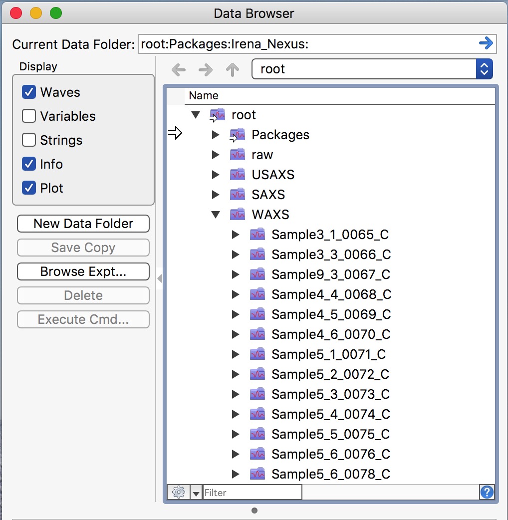
Folders ending in _C contain pinhole-collimated data reduced at the highest possible Q resolution, as required for WAXS.

WAXS data reduction

Data reduction uses the Nika package. Ensure Nika is installed. Select “Load Nika 2D SAS macros” from the Macros menu, or load “USAXS, Irena and Nika” to load all three packages. This creates the SAS2D menu. From the “Instrument Configurations” menu in SAS2D, select “APS USAXS-SAXS-WAXS”. This opens the instrument configuration panel for Nika.

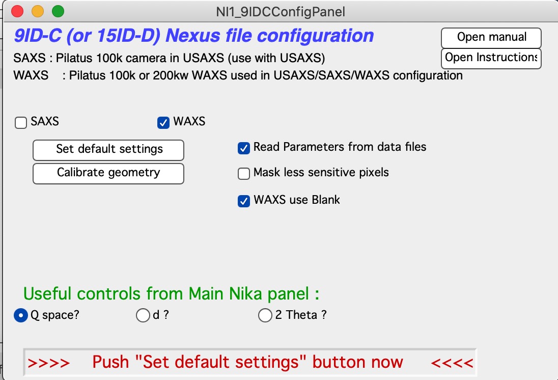
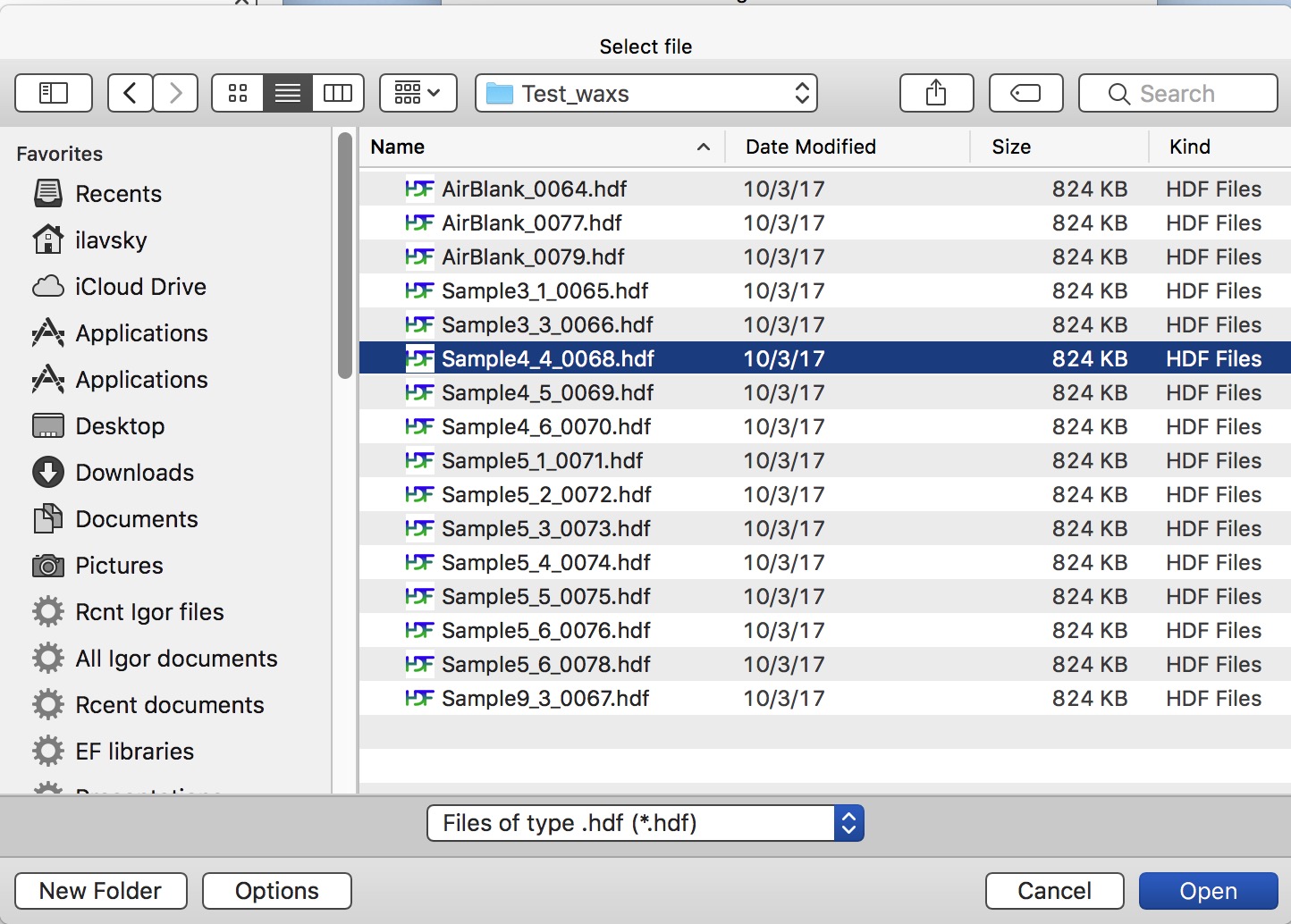
Select (or keep selected) the “WAXS” checkbox and follow the on-screen instructions in red. Keep other checkboxes at their defaults. The first step is to click “Set default settings”, which opens a file dialog. Navigate to your WAXS data folder and select any data file from your samples (assuming no geometry changes within the folder). Click Open.

Nika reads calibration values from the selected file and performs the following steps automatically:

1. All instrument parameters are read and inserted into the appropriate Nika fields.

2. Nika opens the selected image and displays it.

3. Nika sets the correct calibration checkboxes and inserts the appropriate lookup function names for sample thickness, transmission, and normalization.

4. Mask: Depending on the “Mask Less sensitive pixels” checkbox, Nika creates one of two masks. When unchecked (default), a mask covering only the detector edges and the gap between tiles is applied. When checked, pixels between detector chips — which are typically ~1% less sensitive — are also masked. See Impact of different mask selection below.

5. Important: By default, Nika uses Q as the x-axis, which is useful for merging USAXS+SAXS+WAXS data. Two-theta or d-spacing can be selected instead. Note that both the Diffraction tool in Irena and the GSAS-II export function convert any x-axis to two-theta automatically, so the x-axis choice here does not affect downstream use with those tools.

6. Nika displays the Blank selection tab, where you select the appropriate empty/blank file for your samples.

Select the correct blank file — right-click in the panel and use “Match Blank” if needed. Double-click the file or select it and click “Load Empty”.

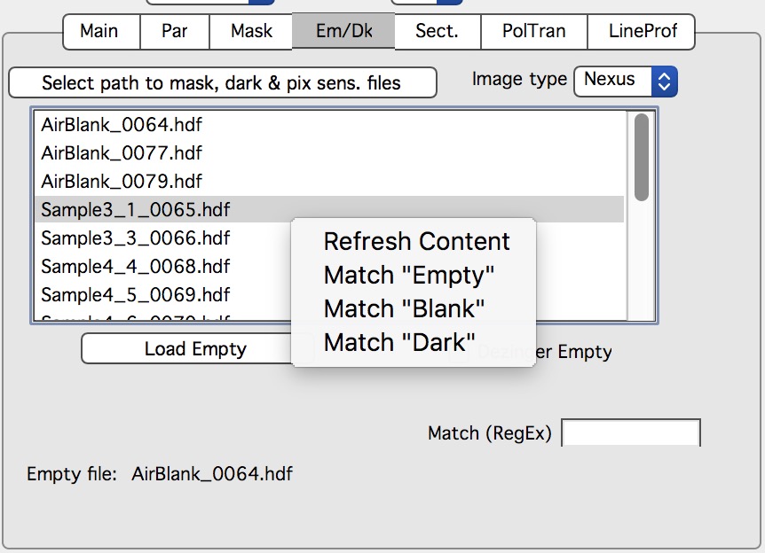
The blank file is loaded and displayed. Select the appropriate blank for each group of samples and update it whenever geometry or sample conditions change.

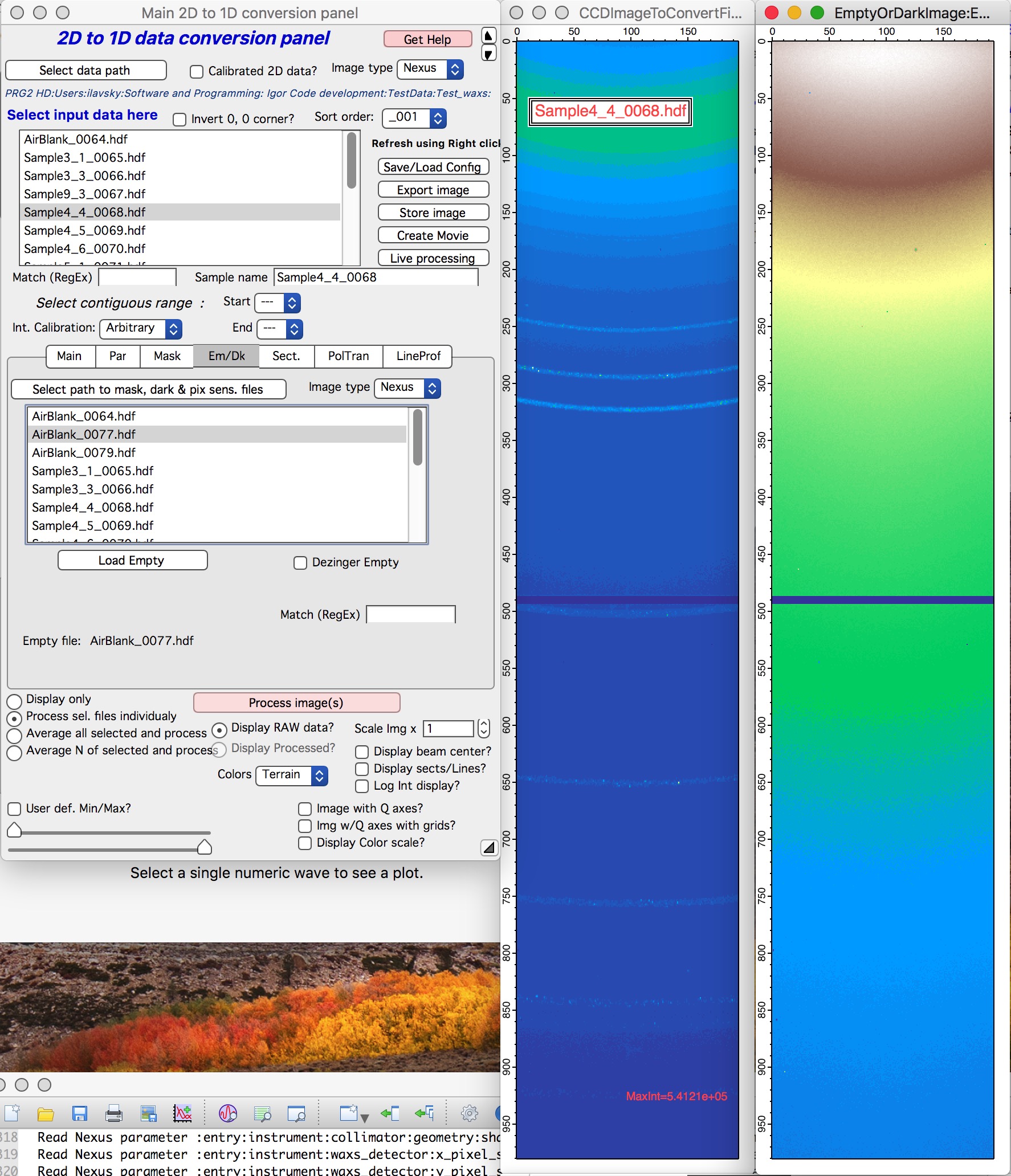
Sample and blank are displayed side by side for comparison.

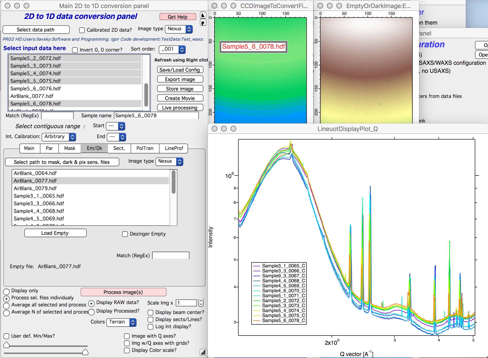
Select the sample file(s) to process and click “Process Images”. Nika processes all selected files.

Impact of different mask selection

Depending on data dynamic range, noise, and overall intensity, pixels at the edges of detector chip tiles can sometimes affect data quality. This is common for Pilatus detectors over time and at certain X-ray energies. Dectris calibrates detector sensitivity at specific energies, but this calibration degrades over time and at other energies. Masking these slightly lower- sensitivity pixels trades Q resolution for data quality. The following image shows data without and with masking of less-sensitive pixels:

And here is how the corresponding mask appears: