Beam Center and Geometry Refinement

The beam center and geometry refinement tool provides the following capabilities:

1. Locate the beam center from an attenuated-beam image by fitting a 2D Gaussian profile.

2. Locate the beam center graphically when diffraction rings are available.

3. Refine the beam center by least-squares fitting to diffraction ring positions.

4. Refine sample-to-detector distance, wavelength, and beam center using a calibrant image (e.g., Silver Behenate for SAXS or CeO for diffraction). User-defined calibrants are also supported.

5. Refine detector tilts. See the tilt section below — this is not straightforward.

Access the tool from the menu: “Beam center and geometry cor.”

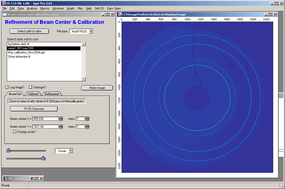
This opens the control panel:

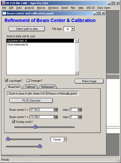
Select the data path and file type. Enable dezingering if needed and set the number of passes. Check “Log image” to display the logarithm of intensity — all calculations use the original (linear) intensity regardless. Click “Make image” to create the image.

If a high-background sample makes diffraction peaks hard to see, check the “Subtr. Blank” checkbox and load a blank image (beam-on, no sample) through the main panel. This subtraction can improve peak visibility.

Additional options: “Use mask?” uses the mask loaded in the main panel (create or load a mask there first). “Use Geom Corrs?” applies geometry corrections to intensity — relevant primarily for very high-angle scattering.

The first tab is for locating the beam center.

Beam center using attenuated beam

Load the attenuated-beam image:

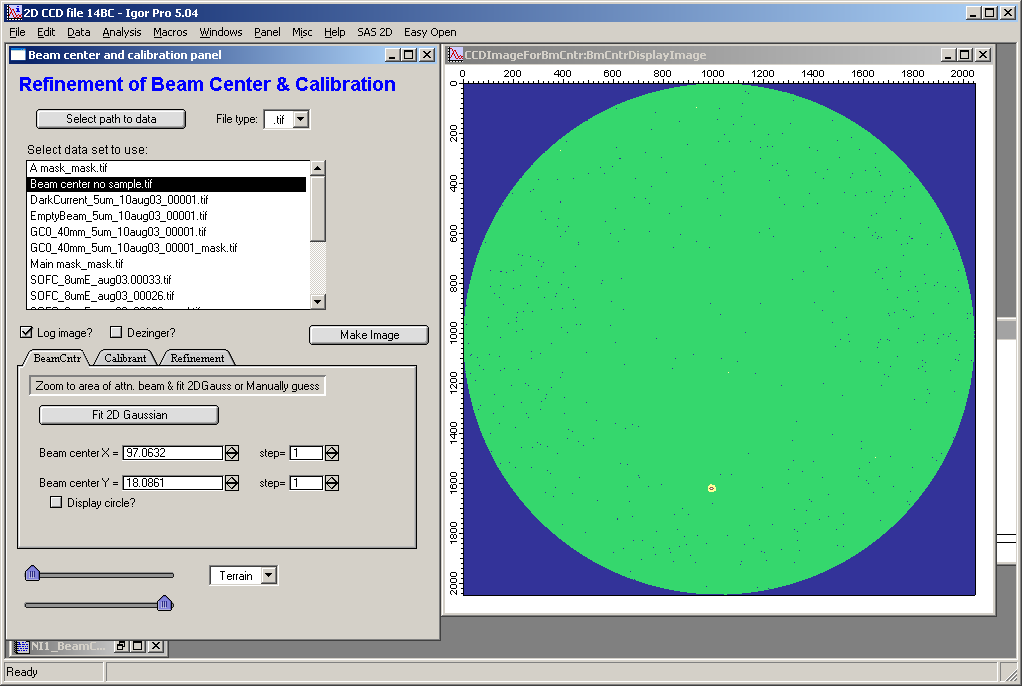
Zoom into the beam region using Igor controls (select the area and right-click → Expand on Windows). Use a reasonably small area — fitting over a large region is slow.

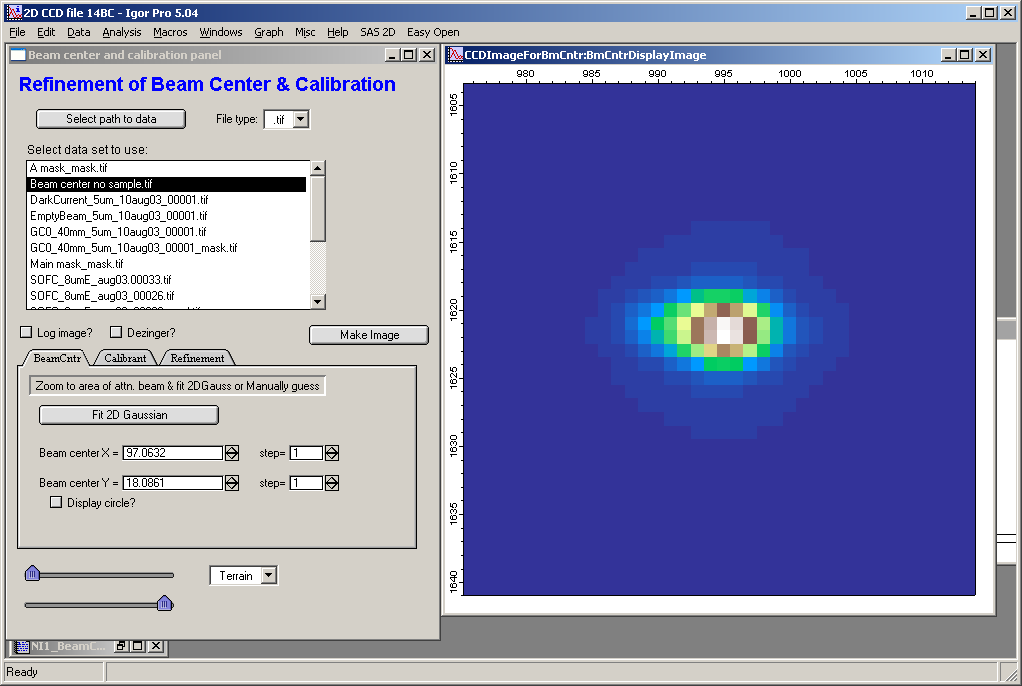
Click “Fit 2D Gaussian”:

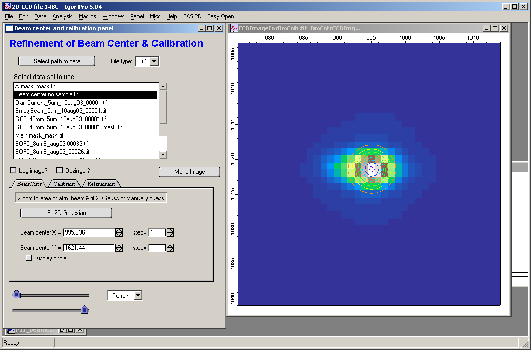
Contours are overlaid on the image showing the Gaussian fit result. The fitted beam center coordinates are automatically transferred to the appropriate variables in the main panel.

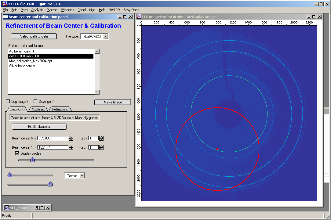
Beam center using “help circle”

If an attenuated-beam image is not available, a calibrant image with diffraction rings can be used to estimate the beam center. Standard calibrants for SAXS include Silver Behenate; CeO and LaB₆ are common for diffraction.

Example: CeO powder standard on a 2D area detector:

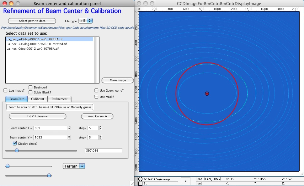
Check the “Display circle” checkbox and use the slider to scale the circle to approximately match one of the rings. Adjust the beam center (set a suitable step size with the “step” controls) until the circle aligns with the ring:

Before adjustment:

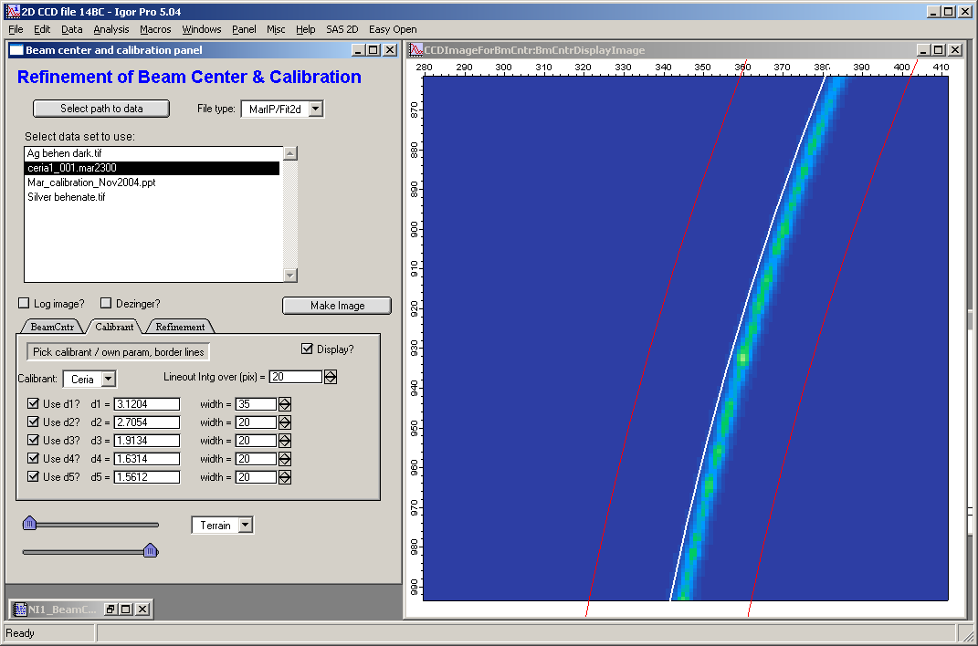
After adjustment:

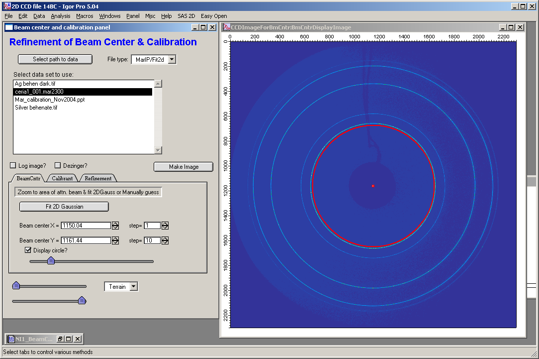
This provides a good initial estimate of the beam center.

Calibrant and refinement

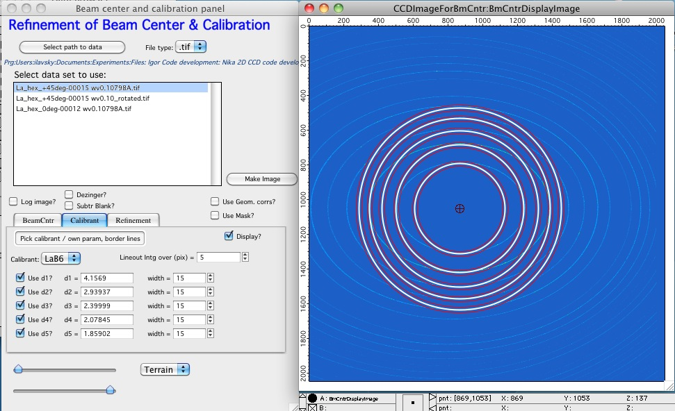
On the Calibrant tab, select the calibrant material and enter reasonable initial estimates for sample-to-detector distance and wavelength on the Refinement tab. Predefined calibrants include CeO and Silver Behenate; additional calibrants can be configured by entering d-spacings directly in the Calibrant tab. The code supports up to 5 diffraction lines per calibrant material. Note that d-spacings are fixed inputs and cannot be refined.

Note

Verify that the correct pixel size is entered in the main panel before running the refinement.

On the Calibrant tab, check the “Display?” checkbox to overlay circles showing the expected positions of the diffraction lines with the current parameters. Two boundary lines (red) indicate the search width used by the refinement code.

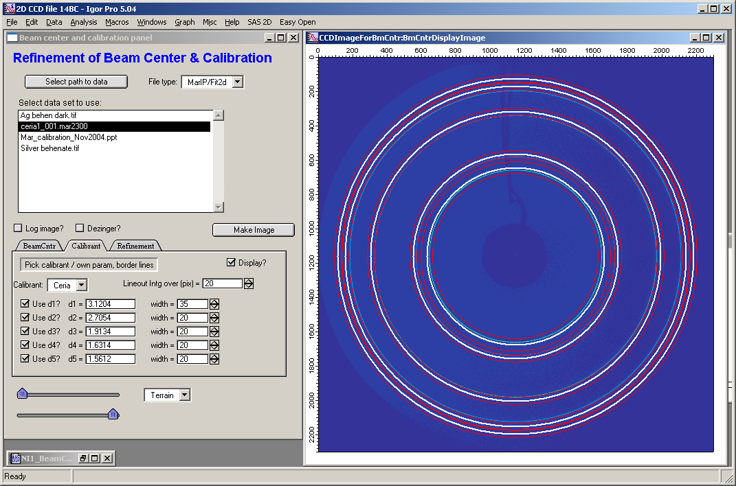
In detail:

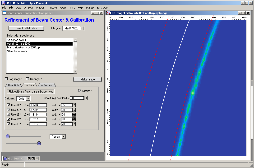
The white line shows the calculated diffraction position; the greenish line is the measured diffraction ring; the red lines show the search boundary. For the refinement to work, the measured ring must lie within the red boundary lines all the way around the circle, and there must be only one ring within the boundary (no overlapping lines). Adjust the wavelength, sample-to-detector distance, and beam center until this condition is met.

Adjust the search width (red boundary lines) per diffraction line as needed. The peak position is found by fitting a Gaussian to the radial intensity profile between the red lines. The fit requires some flat background on either side of the diffraction peak, but should not include neighboring peaks.

The integration width perpendicular to the radial direction (”Lineout Intg. Over (pix)” on the Calibrant tab) applies to all diffraction lines. For broken or spotty rings, a wider integration helps, but reduces precision.

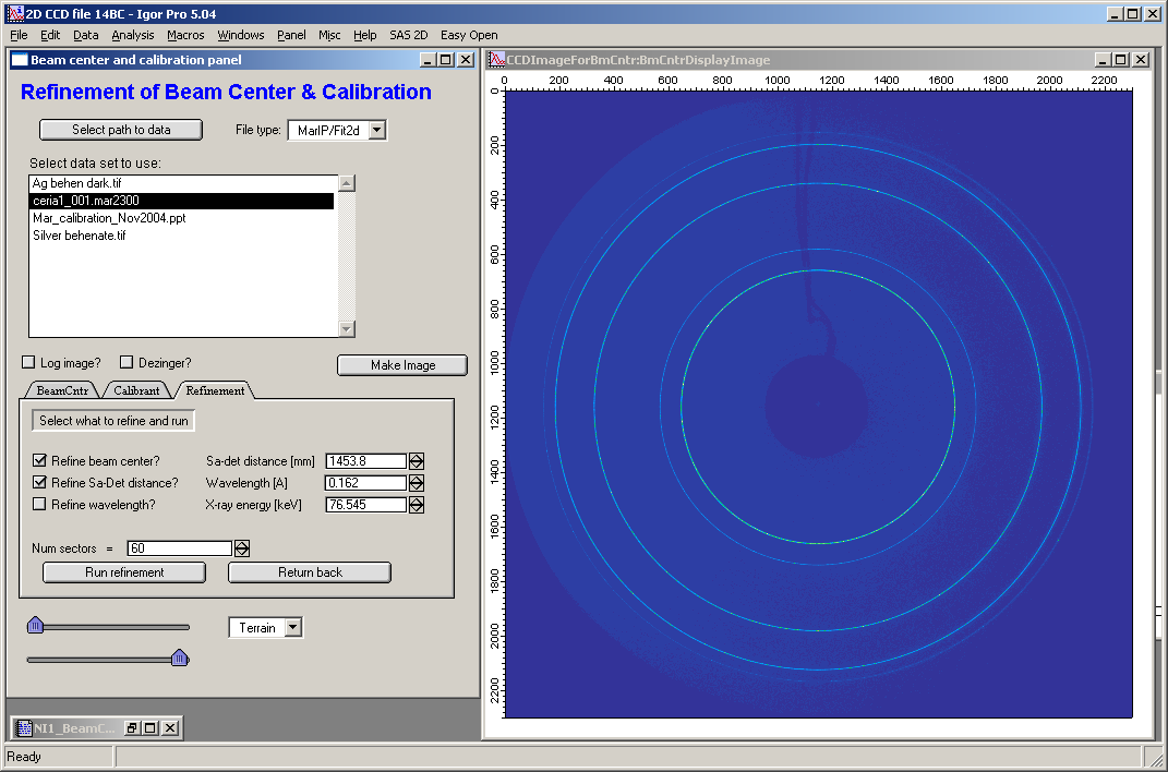
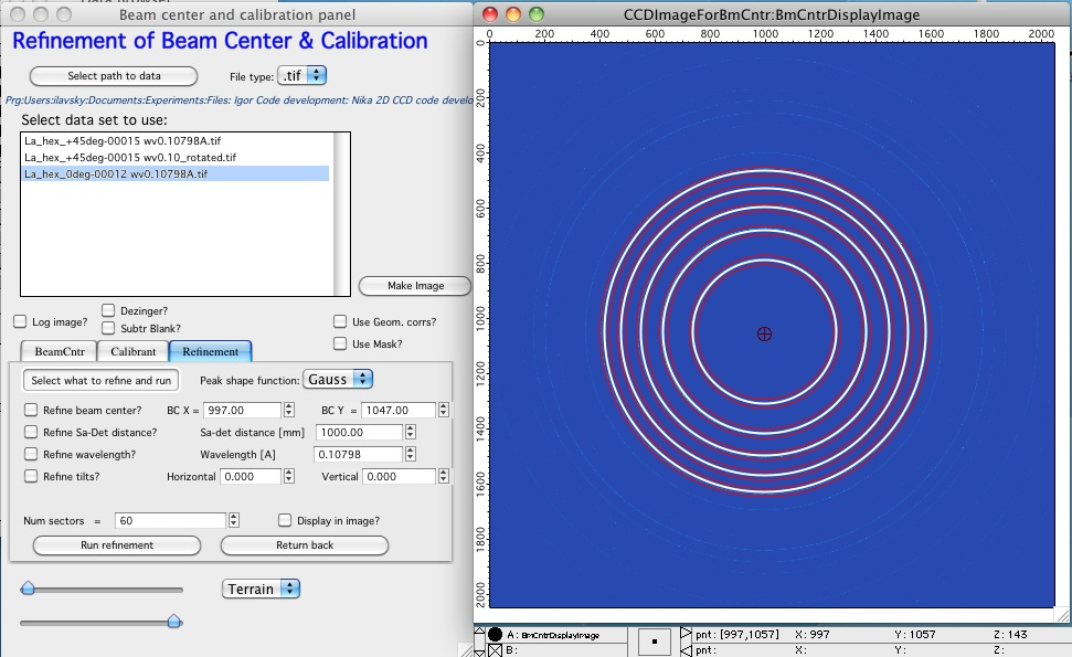
On the Refinement tab, select which parameters to refine: beam center, sample-to-detector distance, and/or wavelength. Note that refining both wavelength and distance simultaneously requires at least two diffraction lines.

Set the number of sectors (radial directions to evaluate). For 60 sectors the code evaluates every 12° (360°/60) around the beam center. For images covering only a fraction of 360° (e.g., when the beamstop or detector edge cuts off part of the ring), increase the number of sectors to ensure sufficient coverage within the available image area.

If the direction of a given sector falls outside the image, it is skipped. Using many sectors increases computation time.

If “Display in image” is selected, the code shows which line is being evaluated in real time. This significantly slows the refinement.

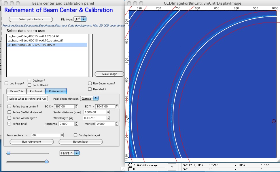
Other refinement controls:

• BC X, BC Y — Beam center coordinates; editable here.

• Peak shape profile — Gaussian (default, most stable), Lorentzian, or Gaussian with sloped background. Alternative profiles are useful when the Gaussian fit fails.

• Tilts — Can be entered or refined; see the tilt section below.

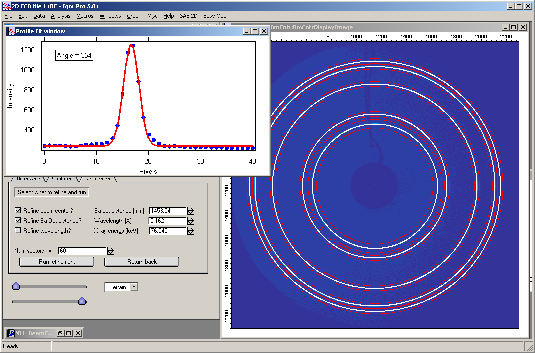
Click “Run refinement” to start. A dotted red line on the image shows the direction being evaluated; the “Profile fit window” shows the intensity profile and fit for each evaluated direction. Poor fits indicate the refinement may produce unreliable results.

If the refinement fails, an error message is displayed and no parameters are changed. If the result is unsatisfactory, click “Return back” to restore the previous parameters.

On successful completion, the refined values are transferred to the main panel.

For Silver Behenate (SAXS calibrant, single diffraction ring): only one diffraction line is available, so wavelength and distance cannot be refined simultaneously. Use a larger line width and lineout integration value for this calibrant.

Fitting data with tilts

Version 1.49 introduced robust tilt fitting for both data reduction and geometry refinement. Earlier versions handled only small tilts. The current implementation handles large tilts accurately and efficiently.

Example: data collected with approximately 45° tilt in one direction:

The diffraction profiles are deformed and resemble (but are not) ellipses.

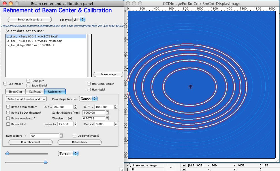
Initial beam center estimate from the circle tool, with known geometry parameters and LaB₆ as calibrant:

The circles do not match the rings well.

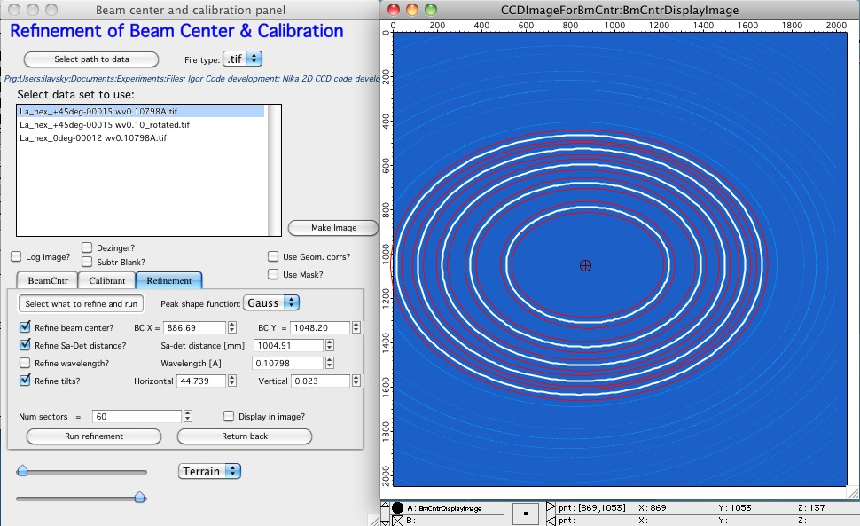
Setting a horizontal tilt of 45° significantly improves the match:

Running the full refinement for beam center, sample-to-detector distance, and tilts gives an excellent result:

Practical notes on tilt fitting:

• Ensure the peak fitting boundaries are wide enough that the refinement does not miss the diffraction ring. Running the refinement multiple times often helps.

• Tilt fitting requires a large solid-angle coverage of data. Fitting tilts with only a small fraction of the diffraction ring visible is generally unreliable. If tilt values are known from external measurements, dial them in manually and verify visually.

• Note that +45° and −45° tilts are physically different (90° apart). If a tilt is known from another measurement, try both signs.

Comparison of data reduced with the correct tilt versus a tilt offset by 5°:

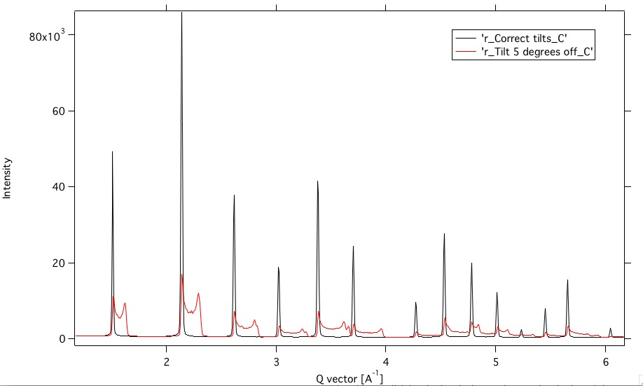
Detector tilts are important for accurate data reduction.