Reduce USAXS Flyscan data in Igor Pro
When using the Indra package to reduce data, the USAXS naming system is
used for compatibility with Irena. When using Irena to analyze, plot, or export
data, select the USAXS option at the top of each panel.
Warning
Save your Igor experiment regularly. Igor Pro is reliable, but no software is crash-proof, and unsaved work can be lost. Develop a habit of saving frequently.
Collected data arrangement
When you collect data on the 12IDC USAXS/SAXS/WAXS instrument, data are saved
in your MM_DD_userName folder. The folder name is formed by prepending the
month and day (MM_DD_) to the name selected by staff, typically based on
the PI username. The folder contains SampleName-level subfolders that can
be created with the command RE(newSample("sampleName")). The default sample
name is "data", used when a newUser command is run.
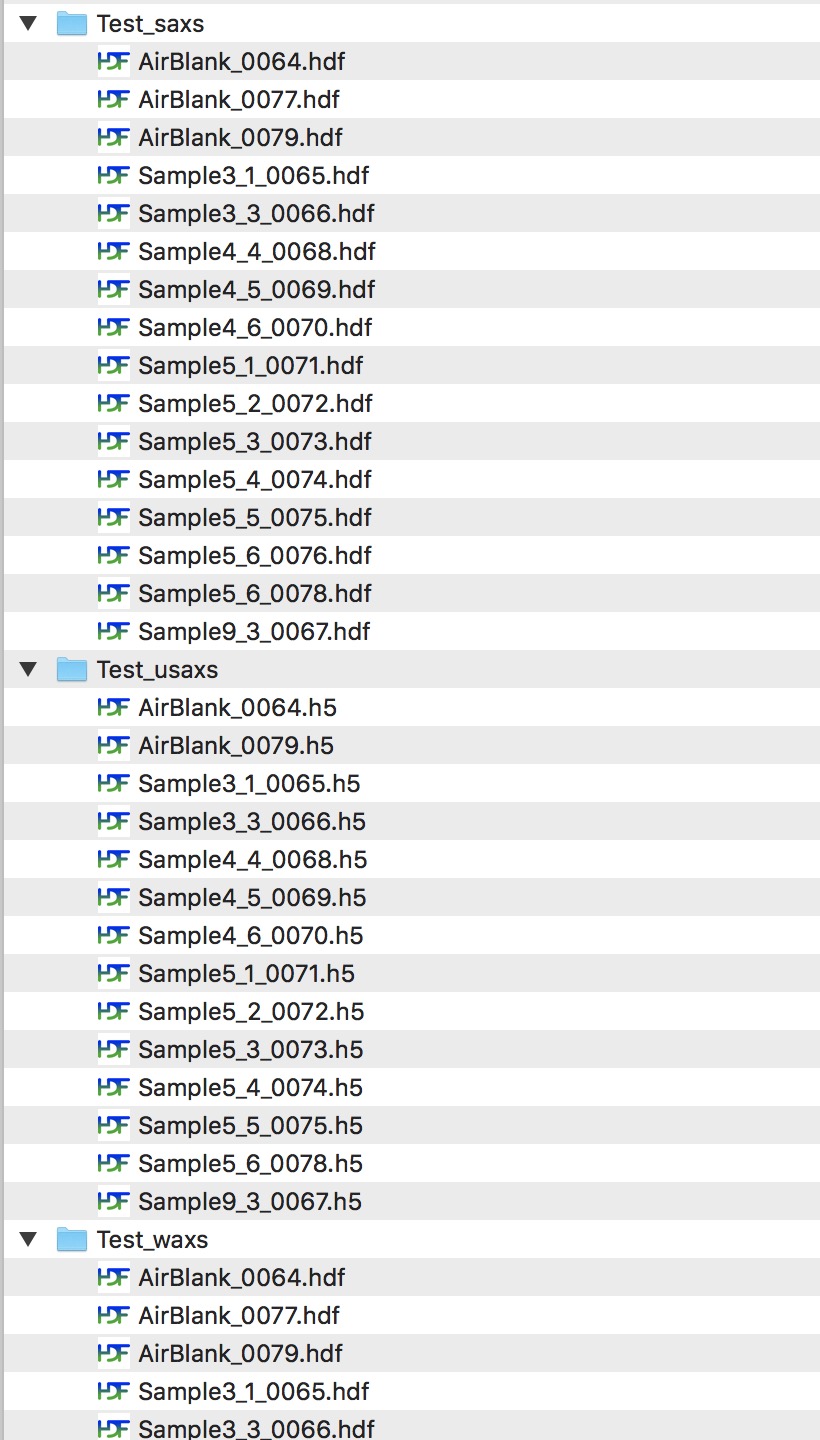
For each data collection type, a subfolder is created with the sample name plus
a suffix: _usaxs for USAXS, _saxs for SAXS, and _waxs for WAXS.
After reducing data, the Igor experiment organizes results in data folders:
USAXS data in root:USAXS:Samplename, SAXS data in root:SAXS:Samplename,
and WAXS data in root:WAXS:Samplename. If a segment was not collected, its
folder may be absent or empty.
When data were collected using the automatically generated or manually entered
script file in the correct order, USAXS, SAXS, and WAXS files will have the
same sample names and the same order numbers (_XYZW suffix) for
measurements that belong together. This correspondence is important for later
data merging.
Reduced USAXS data arrangement
To browse the current Igor experiment, use the Data Browser (Ctrl-B or Cmd-B).
USAXS data (not SAXS or WAXS) are in root:USAXS:Sample_name_Folder.
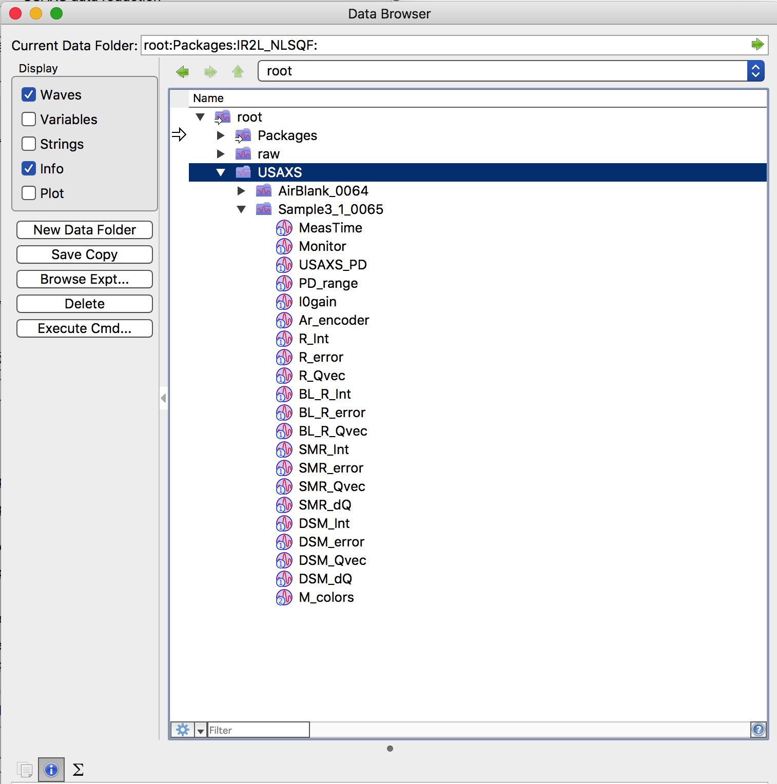
Most waves in this folder can be ignored. The two important sets are:
SMR_Int,SMR_Qvec,SMR_Error,SMR_dQ— Slit-smeared data. Created first; typically on absolute intensity scale with full corrections. Used by Irena for modeling.DSM_Int,DSM_Qvec,DSM_Error,DSM_dQ— Present only if you desmear the data. These are pinhole-equivalent data usable with any SAS analysis software.
Reduce Flyscan data procedure
Flyscanning is the most common USAXS data collection method. If you were not explicitly told that step scanning was used, you most likely collected Flyscan data. If you collected step-scan data, see the separate chapter.
The following procedure covers USAXS data reduction. Subsequent chapters cover SAXS and WAXS data reduction and data merging. SAXS and WAXS reduction uses the Nika package; merging uses Irena.
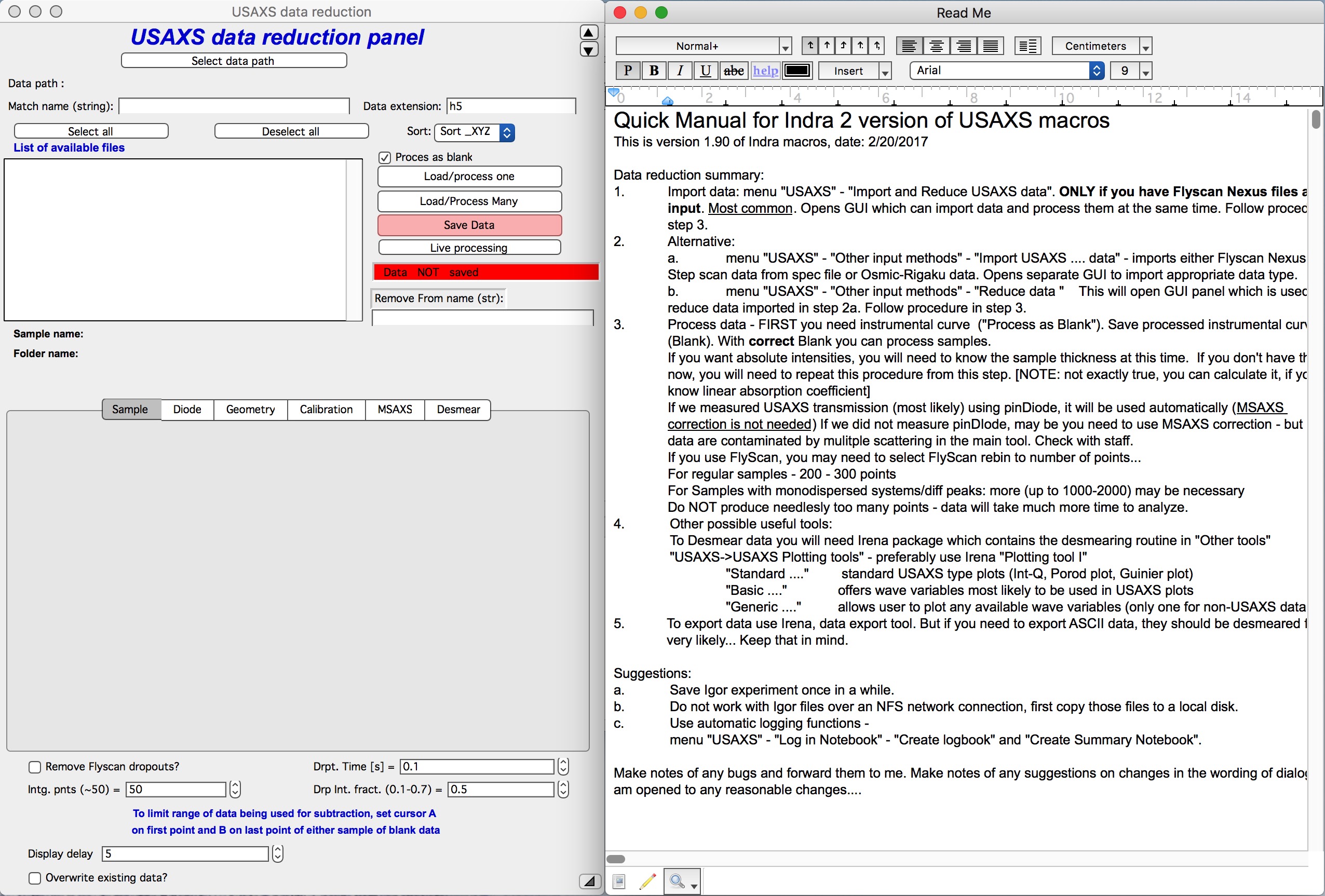
Select “Load USAXS macros” from the Macros menu. This creates the USAXS menu and opens a Read me notebook. Compilation takes a few seconds depending on computer speed. Select “Import and reduce USAXS data” from the USAXS menu.
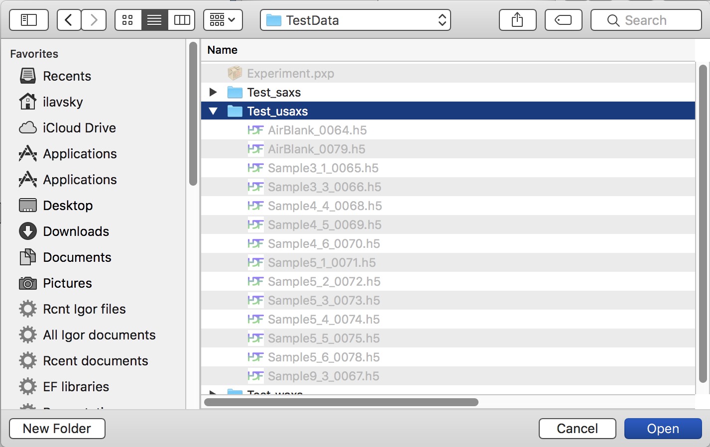
Use “Select data path” to browse to the folder containing the USAXS data
(e.g., TestData/Test_usaxs).
The first step is always to process the instrumental background curve — the “Blank” (also called “Empty” or similar). You must process the Blank before any sample data, because without a valid instrumental curve the sample data cannot be reduced or calibrated. It is critical to use a Blank collected with exactly the same setup and energy, and as close in time to the sample measurement as possible. For samples inside an environment (capillary, heater, etc.), the Blank includes the environment. For capillaries there are two valid Blank choices — an empty capillary or a solvent fill — consult beamline staff for your specific case.
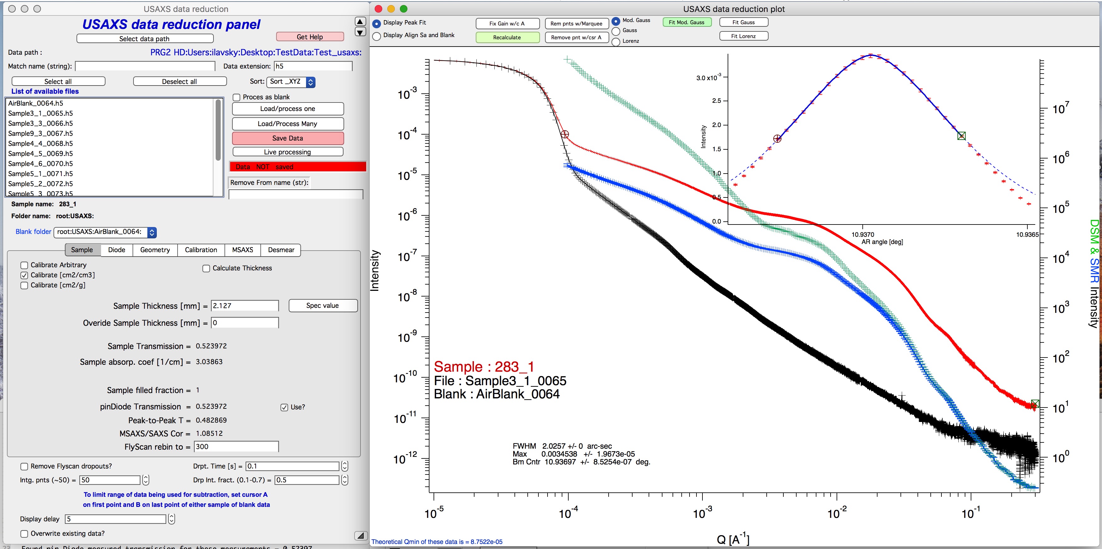
Check the “Process as Blank” checkbox, highlight the Blank measurement in the “List of available files” listbox, and click “Load/process one”.
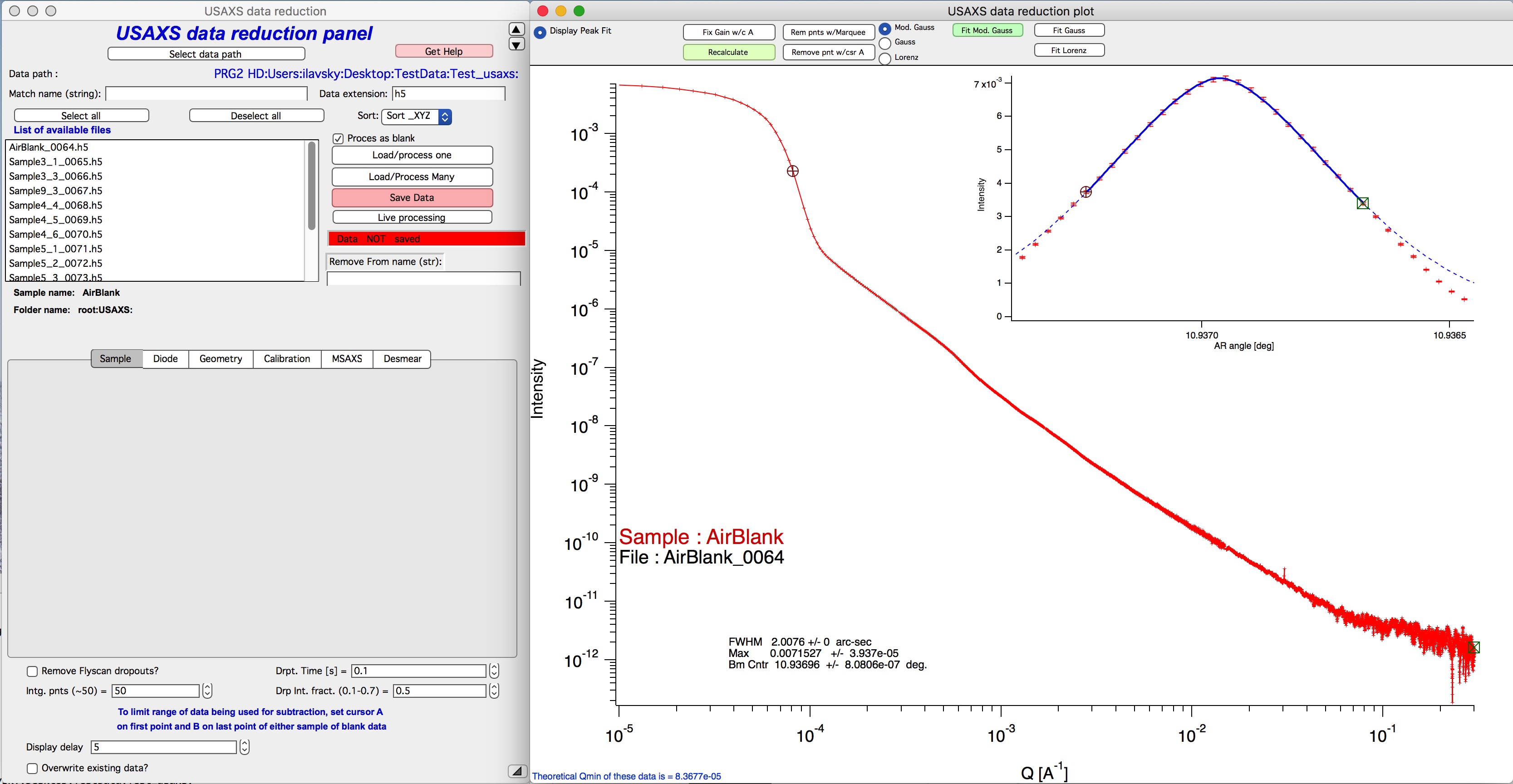
The main graph shows an Intensity-vs-Q plot (log-log). The inset (top-right) shows the same intensity data plotted against analyzer stage angle, fitted with a Gauss+Lorentz function that determines the Q=0 angle, rocking curve width (Q resolution, needed for absolute calibration), and peak maximum (needed for absolute calibration). If the inset fit does not look correct, move the cursors and refit using the available buttons. If the fit continues to fail, contact beamline staff. The main graph shows the instrument background profile, which varies with crystal surface quality and instrument dimensions.
Sometimes you may need to verify diode gain alignment — see the Diode tab discussion below.
Click “Save Data” to store the Blank curve. Then uncheck “Process as Blank” and select the saved Blank name from the “Blank Folder” pull-down menu that appears below the file list. Select a sample in the list box and click “Load/process one”:
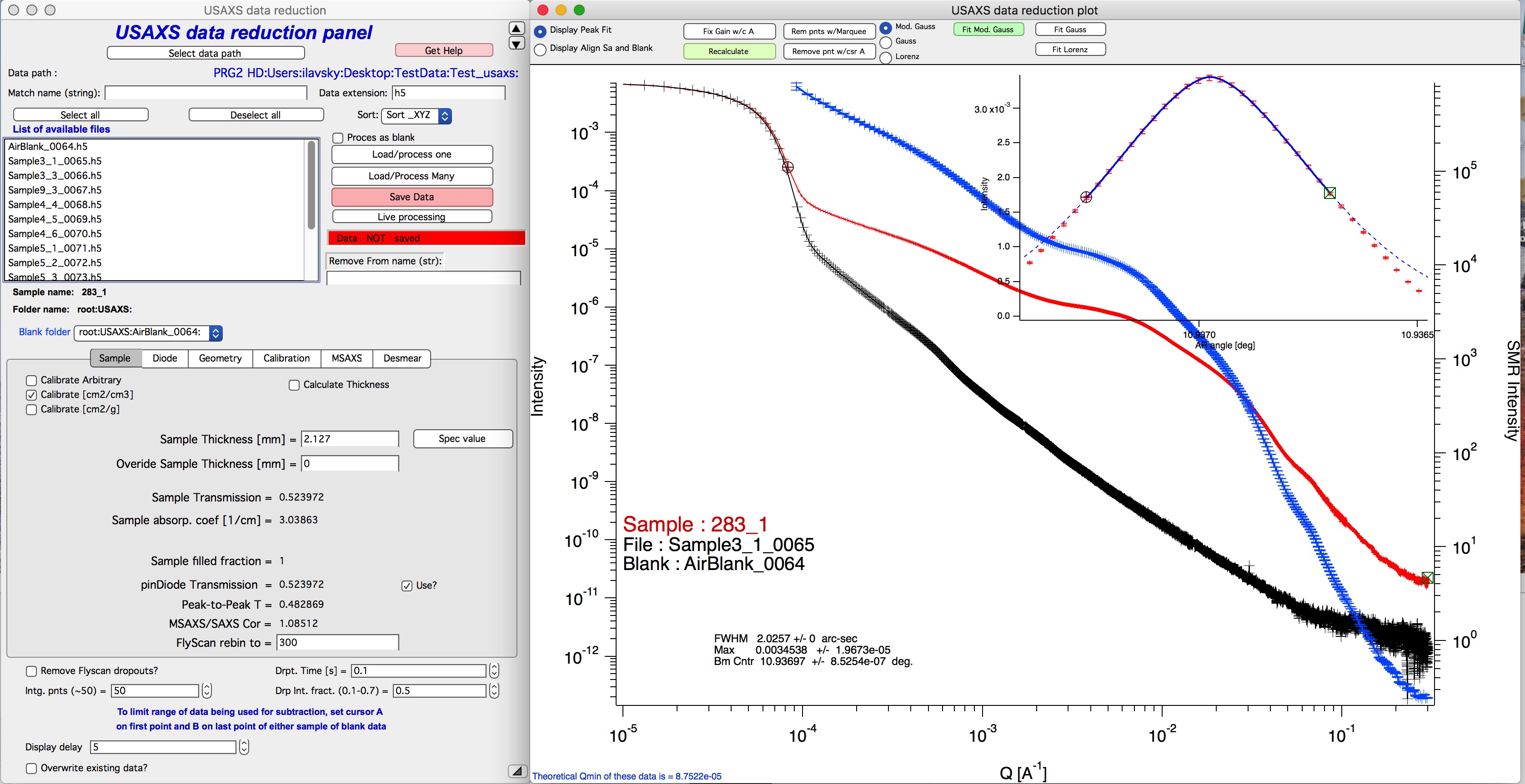
The display shows:
Red curve — sample data scaled by 1/transmission (left axis)
Black curve — Blank data (left axis)
Blue curve — background-subtracted, calibrated, slit-smeared data (right axis)
Inset — peak profile fit for the sample
Check and adjust settings in the following tabs:
Tab Sample
Verify that the calibration method is “Calibrate [cm²/cm³]” if meaningful sample thickness is available. For uncalibrated data select “Calibrate Arbitrary”. For powder samples requiring absolute calibration in units/weight, consult beamline staff — this requires additional steps.
Verify that the sample thickness is correct. If a different thickness is needed, overwrite it here. For many samples with a common non-default thickness, enter the value in “Overwrite Sample Thickness” and it will be applied to all subsequent samples.
Transmission settings should be correct when all transmission measurements agree within 5–10%. Significant variations warrant consultation with staff.
“FlyScan rebin to” — Data are collected at ~8k points over the angular range. For smooth USAXS data, 200–400 points is sufficient. For sharp features (diffraction peaks, Bessel function oscillations), increase to 600–1200 points. Note that noise increases with the number of points.
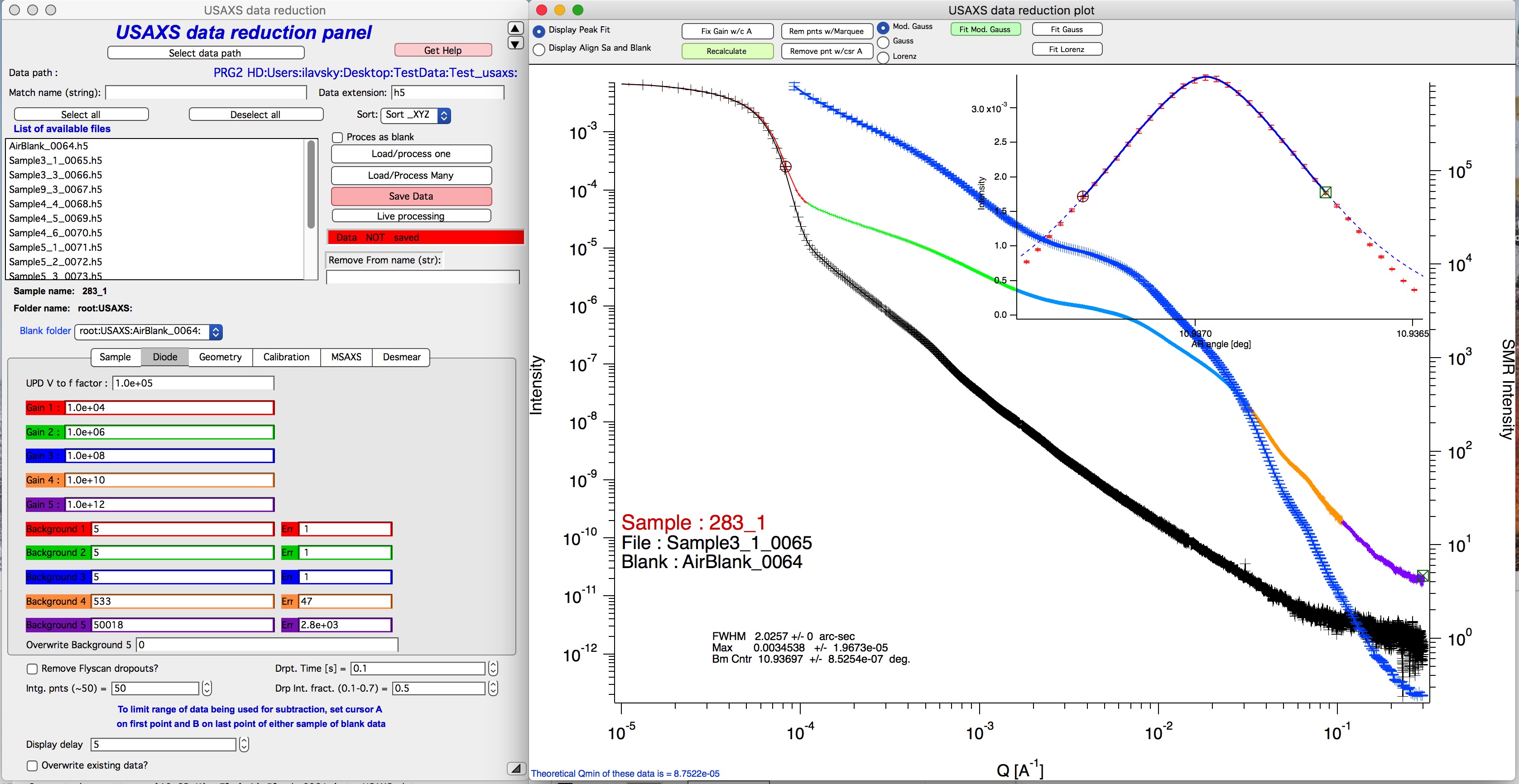
Tab Diode
Most values here do not need changing, except “Background 5” in some cases. If the electronic background and diode dark current differ significantly between sample and Blank — or if the sample has high absorption — you may see sample and Blank data crossing at high Q. In that case, reduce “Background 5” to half or less of the measured value. If this correction is needed for every sample, enter the value in “Overwrite Background 5”.
Check the colored segments in the main graph, which indicate different amplifier gains. If gain transitions are too slow to be correctly removed by the code, check the “Remove Flyscan dropouts?” checkbox and increase the “Drpt. time” value as needed (up to ~1 second in some cases).
Tab Geometry — No changes needed here.
Tab Calibration — No changes needed here.
Tab MSAXS — No changes needed here.
Tab Desmear
If you plan to use any software other than the Irena package for data analysis — including simple plotting or power-law fitting — you must desmear the data first. Other SAS analysis packages do not know how to fit slit-smeared USAXS data correctly.
To desmear, check the “Desmear Data” checkbox. Select the appropriate background extrapolation function (”Background function”) — often “Flat” is correct, but sometimes “Power-law with flat” is needed. The fit to the high-Q data (red dotted line in the lower-right of the main graph, ideally above Q ≈ 0.1 Å-1) shows the result. Adjust the function or the “Background extrapolation start” if needed.
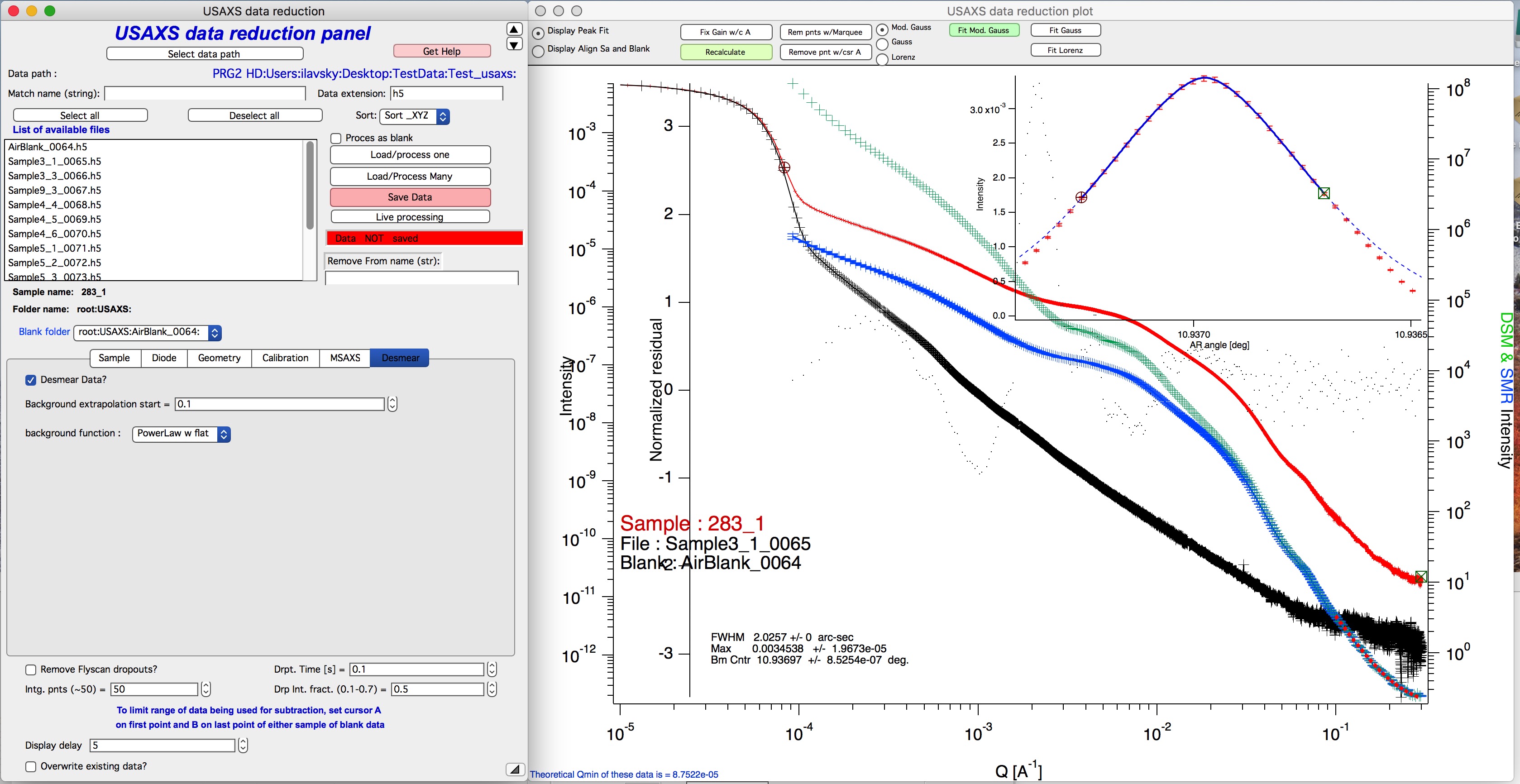
After desmearing, two versions of the corrected data appear:
Blue curve — slit-smeared USAXS data (for Irena)
Green curve — desmeared data (for any SAS analysis tool)
The small dots are normalized residuals from slit-smearing the desmeared data and comparing with the original slit-smeared version. Ideally they are distributed randomly between ±1.
Note
Desmearing always adds noise. Desmeared data will be noisier than the slit-smeared version — if the raw data are already noisy, desmearing may make them unusable. If you plan to use Irena for analysis, desmearing is not necessary, because Irena applies slit smearing to the model internally. For more control over the desmearing process, save the slit-smeared data and use the dedicated Desmearing tool in Irena.
Important — Qmin range check
Warning
This step is critical and sample-specific. Each sample (or group of similar samples) may require a different Qmin setting.
Set cursor A (the round cursor) correctly on the log-log Intensity-vs-Q graph. This defines the starting Q point for background subtraction. The instrumental curve rises steeply at low Q (approximately Q-8), and data near this region have high uncertainties. Select a starting point where the sample intensity clearly deviates from the instrumental background. This is sample-dependent and cannot be automated — choose a point where there is a clearly visible difference between sample and Blank.
Check for multiple scattering. Many samples (particularly powders) exhibit multiple scattering, which can be identified by comparing the FWHM of the rocking curve peak fit for the sample versus the Blank. If the sample FWHM is more than ~20% wider than the Blank, consult beamline staff.
If the warning “Warning — too small Qmin detected. Reset to calculated Qmin = …” appears, cursor A was positioned too far to the left and has been automatically moved right. This check runs only when “Load/process one” is clicked.
The cursor A position is remembered between samples and is never moved leftward automatically. Check its position for each new sample, as the appropriate Qmin depends on the sample’s scattering strength.
When satisfied with the result, click “Save Data”. A new graph is created showing the final Intensity-vs-Q curve (desmeared if desmearing was selected, slit-smeared otherwise). This graph can be closed; it is recreated as needed.
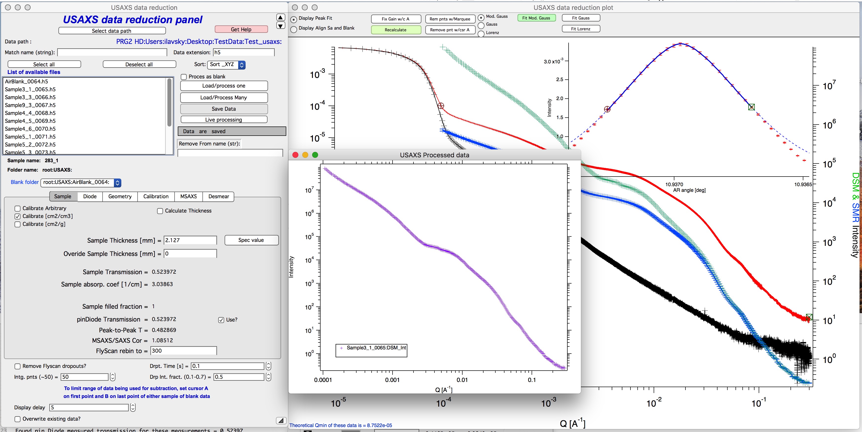
Proceed to process the remaining samples.