Analytical models — obsolete

Note

This tool has been superseded by System Specific Models. Use that tool for new work.

This tool provides a GUI for three models: Debye-Bueche, Treubner-Strey, and Ciccariello-Benedetti. All models can be combined with a low-Q single Unified level. The panel has four tabs: one for the Unified level, and one each for the three models. Combining models is possible but is unlikely to be physically meaningful.

For the Unified level controls, see the Unified Fit documentation. Version 2.54 added the ability to link RgCO to parameters from the Debye-Bueche and Treubner-Strey models, and added a residuals plot.

Debye-Bueche model for gels

The Debye-Bueche model is implemented as:

\[I(q)=\frac{4\pi K \varepsilon ^2 \xi^3}{(1+Q^2\xi^2)^2}\]

where \(K = 8 \pi ^2 \lambda^{-4}\), ξ is the correlation length, and ε is the mean-square fluctuation parameter.

The model also allows fitting and subtraction of a low-Q power-law slope and a flat SAS background.

Note

In August 2012, a user identified that the original implementation used ξ² in the numerator rather than ξ³. Based on available citations (Hammouda, NIST), the correct formula uses ξ³. The source of this discrepancy (dating to approximately 2003) is under investigation. If you have a definitive citation on the correct form, contact the developer.

The standard Debye-Bueche model from Hammouda (NIST) is:

The pair correlation function (Debye-Bueche, 1949):

\[\gamma(r) = \exp\!\left(-\frac{r}{\xi}\right)\]

Scattering cross section:

\[\frac{d\Sigma(Q)}{d\Omega} = \frac{C}{\left[1+(Q\xi)^2\right]^2}\]

where the prefactor is:

\[C = 8\pi\Delta\rho^2\phi\xi^3\]

The Debye-Bueche model is a special case of the Teubner-Strey model for very large d-spacing (d >> ξ).

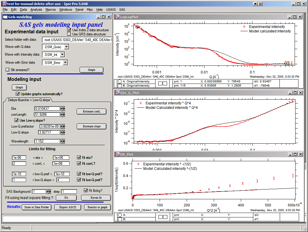
Main screen:

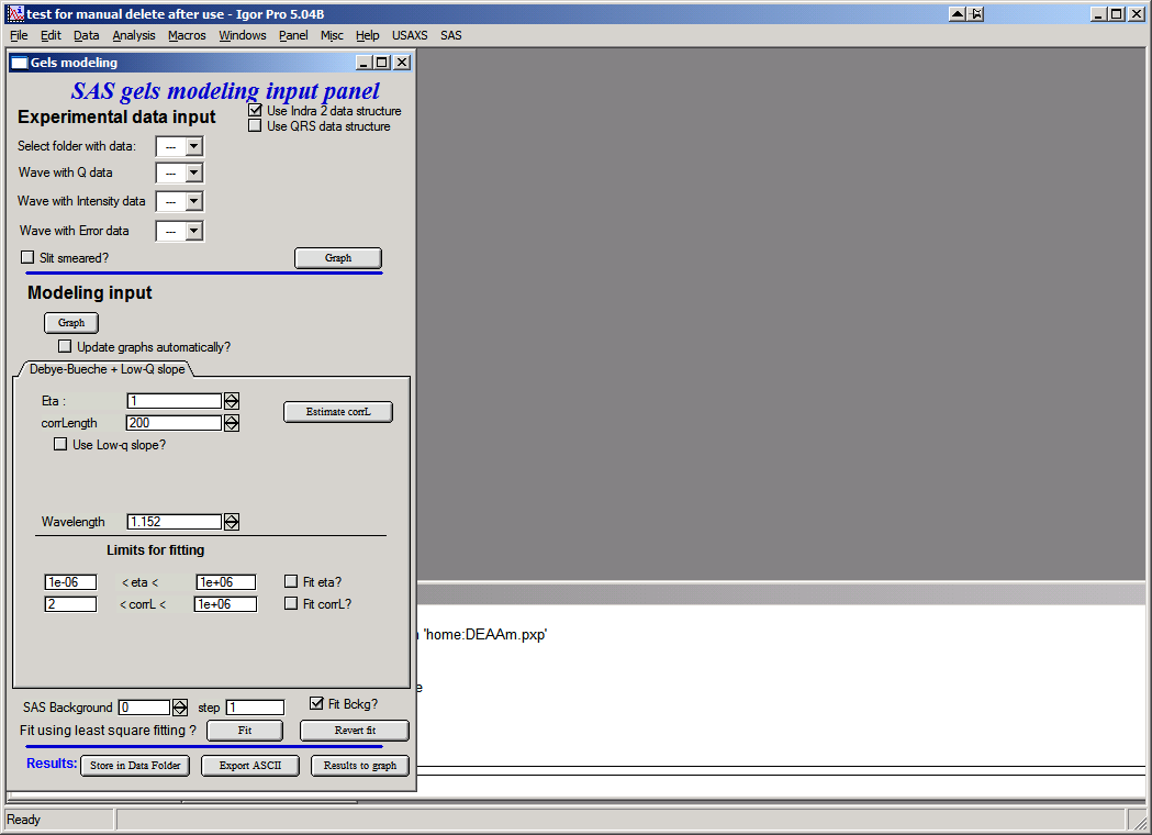
The top section contains standard data selection tools. Both pinhole (or desmeared USAXS) and slit-smeared data are supported; the model is slit-smeared internally when slit-smeared data are used.

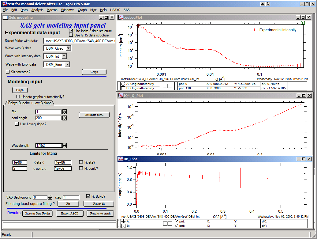
Data loaded and graphed: top is log-log, middle is I × Q⁴ vs Q, bottom is 1/√(Intensity) vs Q². Data range selection for fitting is done in the top graph only.

Controls:

“Graph” (top) — loads data and creates the graphs.

“Graph” (lower) — calculates the model and adds it to the graphs.

“Update graphs automatically” — recalculates the model after any parameter change. Recommended for fast machines.

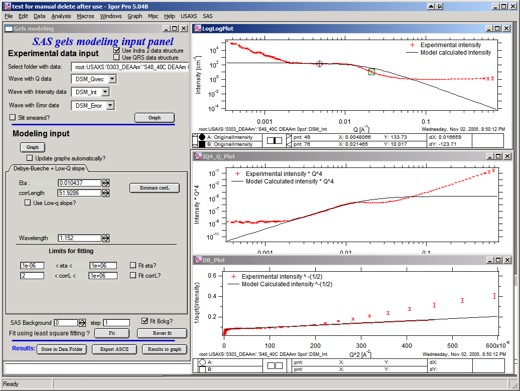
“Eta” and “corrLength” — model parameters. Click “Estimate” after selecting the Guinier knee region in the top graph to obtain initial estimates:

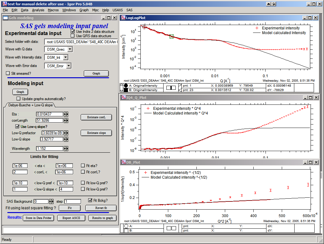
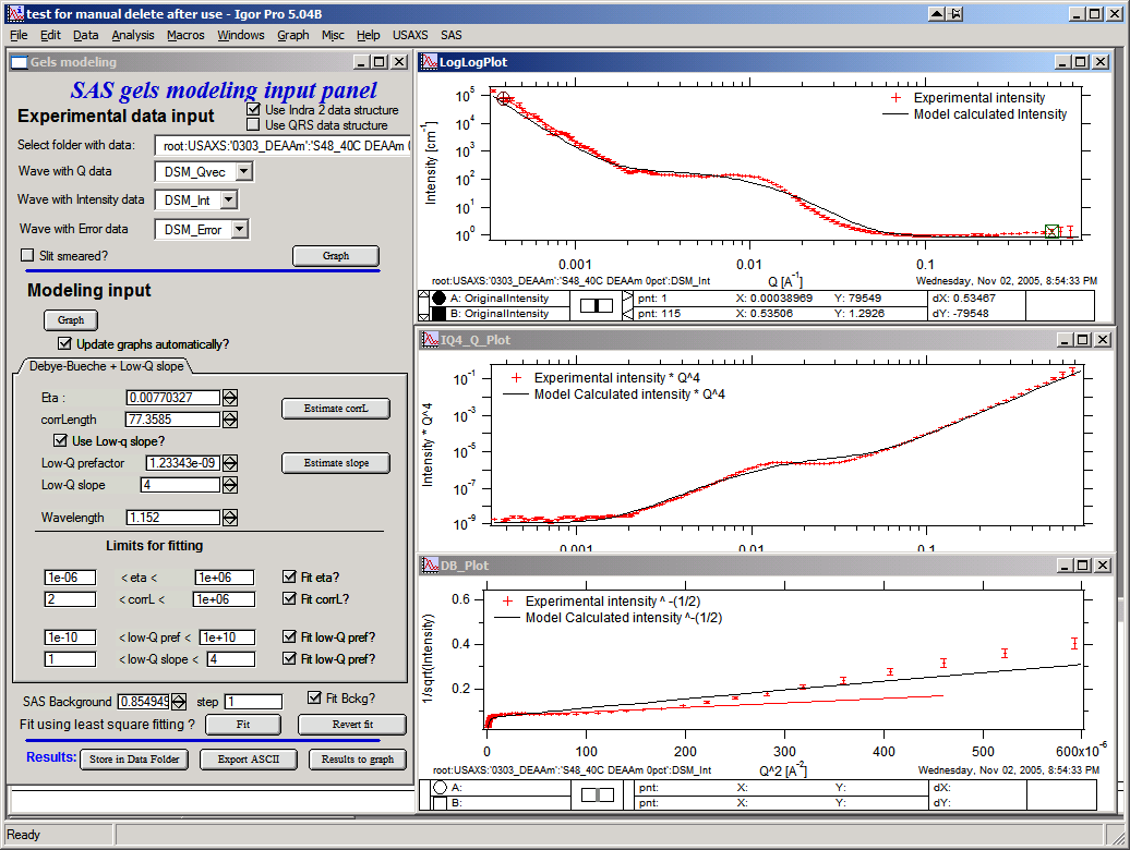
“Use low-q slope” — enables controls for a low-Q power-law slope. Select the appropriate Q range and click “Estimate” to fit initial values:

“Limits for fitting” — set sensible bounds before fitting.

“Background” — estimate a starting value, then fit as a free parameter:

Fit the model with the “Fit” button:

Buttons:

“Revert fit” — restores the last set of parameters after a failed or divergent fit.

“Store in Data folder” — copies model waves (with wave notes) to the source data folder. Results can be plotted, exported, reloaded, and mined for values.

“Export ASCII” — exports the model as ASCII from Igor.

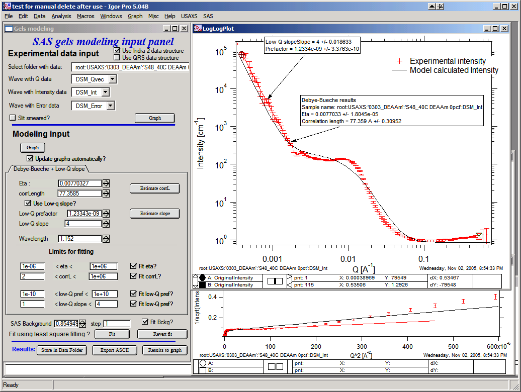
“Results to Graph” — overlays fit parameters as text in the graph:

Treubner-Strey for small-angle diffraction

References:

• Teubner, M.; Strey, R. J. Chem. Phys. 1987, 87, 3195.

• Schubert, K-V.; Strey, R.; Kline, S. R.; Kaler, E. W. J. Chem. Phys. 1994, 101, 5343.

The code is adapted from the NIST SANS package. The model:

\[I(Q) = TS\frac{1}{A + C_1 Q^2 + C_2 Q^4}\]

where A, C₁, and C₂ are theory parameters and TS is a scaling factor. Correlation length ξ and repeat distance d are:

\[ \begin{align}\begin{aligned}\xi = \left[\frac{1}{2}\left(\frac{A}{C_2}\right)^{0.5} + \frac{C_1}{4C_2}\right]^{-0.5}\\\frac{d}{2\pi} = \left[\frac{1}{2}\left(\frac{A}{C_2}\right)^{0.5} - \frac{C_1}{4C_2}\right]^{-0.5}\end{aligned}\end{align} \]

Only TS, A, C₁, and C₂ are user-controlled. TS is a scaling factor required to match the model amplitude to the data.

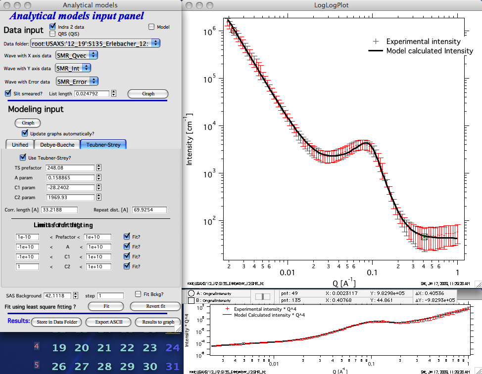
Example fit to slit-smeared data appropriate for the Treubner-Strey model.

Ciccariello-Benedetti model for coated smooth surfaces

References:

• Benedetti, A.; Ciccariello, S. “Coated Silicas and Small-angle X-ray intensity behavior,” J. Appl. Cryst. (1994) 27, 249–256.

• Pikus, S.; Kobylas, E.; Ciccariello, S. “Small-angle scattering characterization of n-aliphatic alcohol films adsorbed on hydroxylated porous silicas,” J. Appl. Cryst. (2003) 36, 744–748.

This model assumes a constant-thickness, constant-SLD coating on the surfaces of a porous medium, where the film surface is always parallel to the solid surface. It is a modification of Porod’s law: the interface must be sharp, so the Porod Q^-4 slope is modulated by an oscillatory term from which the film thickness and contrast can be extracted.

Note

Discrepancies have been observed between results using finite slit length (with Irena’s internal slit-smearing routines) and infinite slit-length approximations. Results depend on the assumed slit length — read carefully before use.

Control panel:

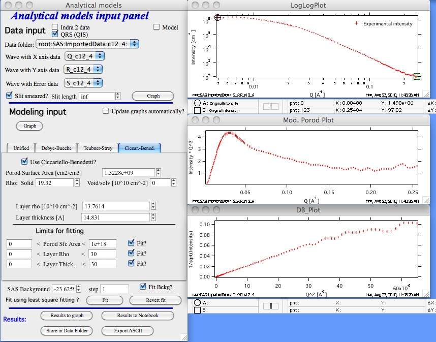
This is the only Irena tool that supports both finite slit length and “inf” (infinite slit length) for the slit-smearing correction. Pinhole data are also supported.

Enable the “Use Ciccariello-Benedetti” checkbox to reveal the model controls.

Model parameters that can be fitted:

• Porod specific surface area — area of the solid/void interface (without the coating layer).

• Layer SLD (scattering length density of the coating layer).

• Layer thickness.

Known/fixed parameters:

• Solid SLD — scattering length density of the solid phase.

• Void SLD — scattering length density of the void/solvent (typically 0 for air).

Set the SAS background and fitting limits, and enable the “Fit?” checkboxes as in other Irena tools.

Clicking “Graph” generates three plots:

1. Intensity vs Q — the only graph on which the fitting range can be selected.

2. Intensity × Q⁴ (or Intensity × Q³ for slit-smeared data).

3. 1/√(Intensity) vs Q².

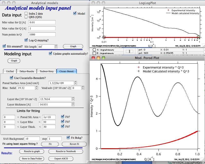
To visualize an ideal system, run the tool in “Modeling” mode without loading input data (use model-generated data only):

Slit-smeared example:

Pinhole-collimated example (same parameters):

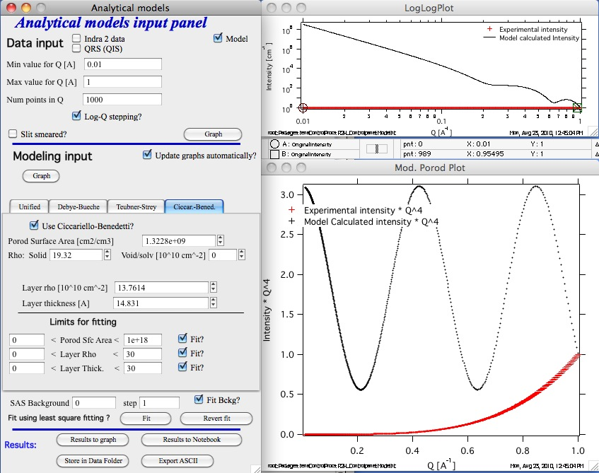
Note that for pinhole data the lower graph shows Intensity × Q^-4.