Evaluate size distributions
This tool obtains various details about size distributions, such as results from the Size Distribution, Modeling I, and Modeling II tools. You can calculate mean, mode, and median size within a cursor-selected range, as well as volume, surface area, and particle number density (per cm3). The tool can also generate cumulative distributions and mercury intrusion porosimetry (MIP) curves showing intruded volume as a function of pressure (in psi).
Multiple size distributions can be displayed simultaneously, though the graph becomes crowded quickly.
Description
Select “Evaluate size distributions” from the SAS menu.
All controls are located in the control bar at the top of the graph window. For MIP data, a new window opens automatically. Monitor the history area for important messages about tool requirements and events.
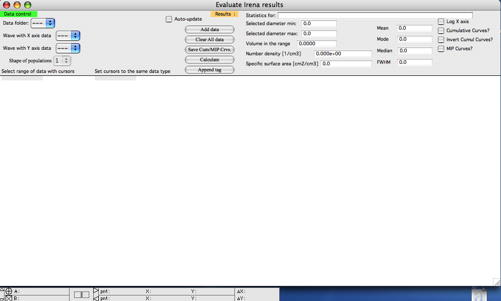
Data selection controls (top left)
This tool recognizes all Irena result data types suitable for analysis. Select a data folder; you will see only folders containing at least one useable data type. If multiple data types exist in a folder, select the appropriate ones. You may need to specify both X-axis and Y-axis data. Minimal validation is performed, so verify your selections carefully.
The “Shape of populations” popup (initially grayed) is described below.
Results area
“Statistics for:” displays the name of the dataset on which cursors are positioned and for which calculations are performed.
“Selected diameter min” and “max” show the diameters at the current cursor positions.
“Volume in the range” — The fractional volume of scatterers between the cursors, calculated using the appropriate formula for the form factor.
Note
For distributions from Modeling I and II, the code cannot automatically determine which volume formula to apply to mixed-shape populations. When combining different shapes, accurate calculations of volume and particle number are problematic. To address this, the “Shape of distributions:” popup becomes available, allowing you to select which shape formula to use. This is meaningful only when populations are well separated and their spatial distribution is known.
When using a volume distribution, the volume value is always correct (no conversion required), but particle number may be incorrect.
When using a number distribution, particle number is correct, but volume may be incorrect.
Specific surface area is likely affected unless the correct shape is selected.
You will be informed of ambiguity via a message in the history area:
“These data may contain mixture of shapes for different populations. Please select the right population number to evaluate.”
This limitation does not apply when individual distributions are saved alongside the total distribution and evaluated together; the code automatically selects the correct shape for accurate calculations.
“Number density” — Number of particles per cm3 in the cursor range.
“Specific surface area” — Specific surface area between the cursors.
“Mean”, “Mode”, “Median” — Values calculated numerically for the given distribution within the cursor range. Note that these differ between number and volume distributions.
“FWHM” — Full width at half-maximum, evaluated numerically. This metric is meaningful only for single-peak distributions. While a value is always provided, it may not be useful for multimodal data.
Display options
“Log X” — Sets the diameter axis (x-axis) to logarithmic scale.
“Cumulative curves” — Calculates and displays cumulative curves.
“Invert Cumul. Curves” — Forces the origin (zero) to occur at large sizes. Useful in certain analytical scenarios.
“MIP curves?” — When selected, calculates MIP curves and opens a new window displaying them. Additional controls appear for MIP parameters:
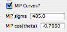
These parameters control MIP calculations and use standard values, which you can modify as needed. Sigma is in dynes/cm; cos(θ) is dimensionless, where θ is the wetting angle between the material and mercury.
Example
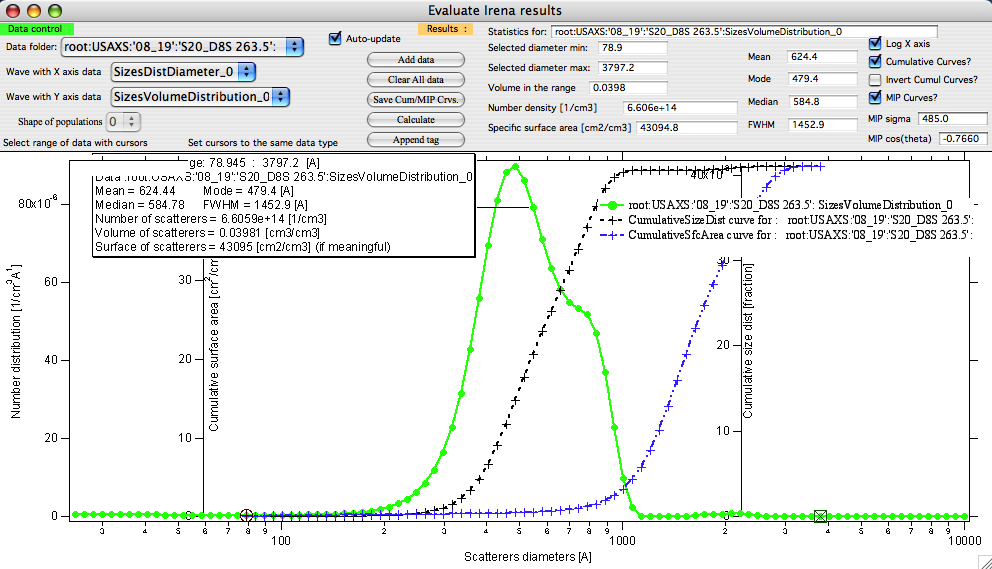
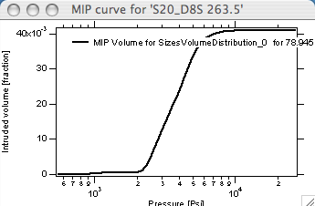
In this example, the green curve shows original data with cursors selecting the evaluation range. The black curve is the cumulative size distribution by volume (right axis), and the blue curve is cumulative specific surface area (left axis). The tag displays a results summary. Because the MIP curves checkbox was selected, an additional MIP graph was generated:
Saving the data stores both cumulative curves and MIP curves in the original data folder for export or future use.
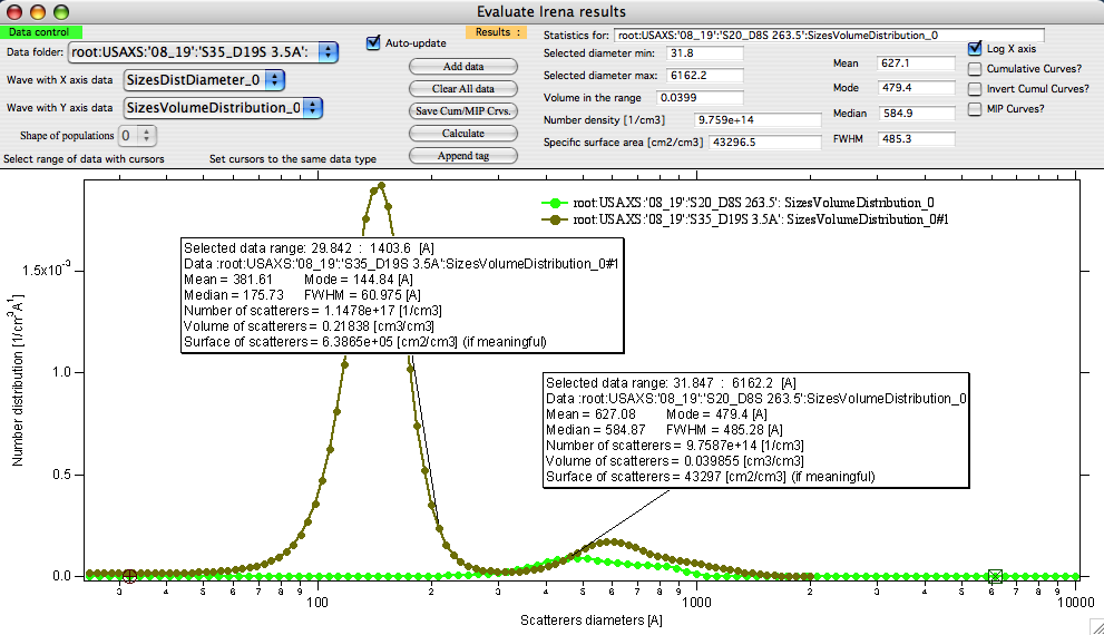
Example of comparing two datasets and using tags to display results for both:
New data created
When you save cumulative and/or MIP curves, new data are created in the folder containing the original size distributions. These are named:
MIPVolume_XXMIPPressure_XXCumulativeSizeDist_XXCumulativeSfcArea_Dist_XXCumulativeDistDiametersDist_XX
where XX is an index ensuring uniqueness.
The indexing logic is as follows:
The code first attempts to use the index from the original data. For example, if the original data is
SizesVolumeDistribution_2, it checks whether index 2 is available. If so, the data is saved with that index, and the result is printed in the history area.If the index is already in use, a message alerts you, and the index is incremented. Track the correct index to know which saved curves correspond to which input data.
The history area prints what data were created and in which generation they were saved. Example output:
Saved Cumulative data to CumulativeSizeDist_02 / CumulativeSfcArea_Dist_02
/ CumulativeDistDiametersDist_02 in folder root:USAXS:'08_19':'S20_D8S 263.5':

Saved MIP data to MIPVolume_01 / MIPPressure_01 in folder
root:USAXS:'08_19':'S20_D8S 263.5':
The waves contain descriptive wave notes that can be exported as ASCII header information or searched using the Data miner tool.