Two Phase Solid model
This tool generates a 3D random representation (voxelgram) of a two-phase solid material using the method implemented in SAXSMorph. For details on the underlying science, see:
B. Ingham, et al., “SAXSMorph: a program for generating representative morphologies for two-phase materials from small-angle X-ray and neutron scattering data,” J. Appl. Cryst. 44 (2011) 221–224. https://doi.org/10.1107/S0021889810048557
J. Quintanilla, “Versatility and robustness of Gaussian random fields for modeling random media,” Modelling Simul. Mater. Sci. Eng. 15 (2007) S337–S351. https://iopscience.iop.org/article/10.1088/0965-0393/15/4/S02/meta
Warning
This model is applicable only to two-phase solid materials. It generates one of many possible 3D arrangements consistent with the measured scattering curve; it is a visualization tool, not a unique solution. The back-calculated intensity from the generated structure is compared to the input data.
Practical resolution (size/voxel size) is approximately 100 on a modern computer (150–200 may be achievable with sufficient memory and time). This limits the modeled range of scatterer sizes to roughly 20–40, constraining the usable Q range to approximately 1 to 1.5 decades.
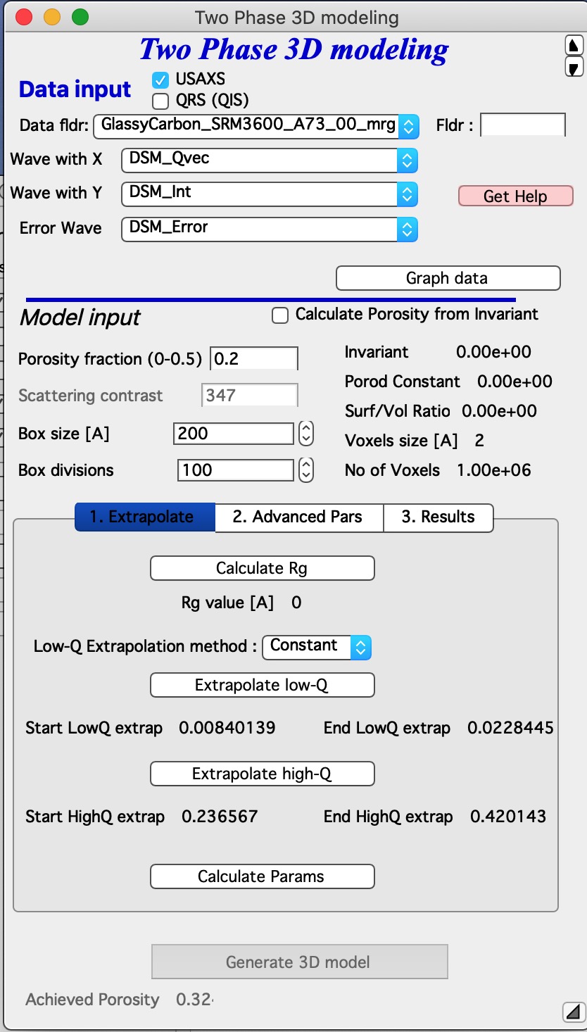
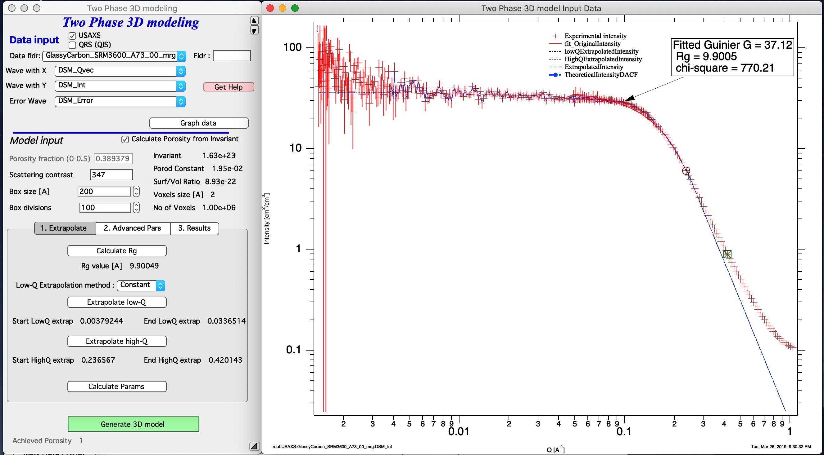
The top section contains standard data selection tools. USAXS data used with this tool must be desmeared.
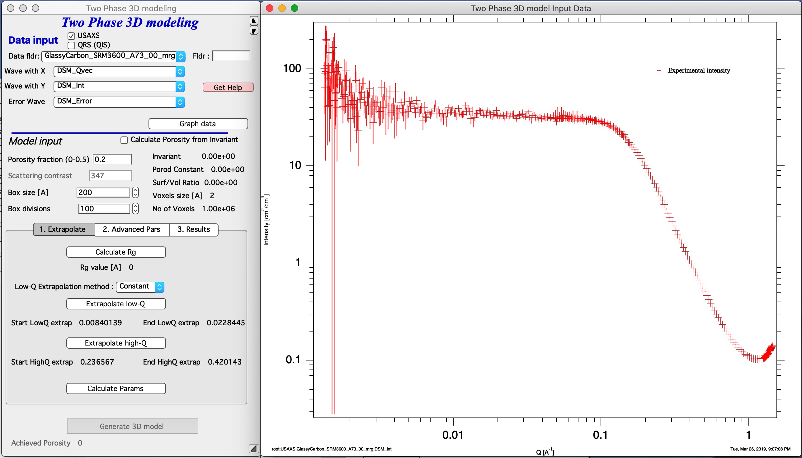
Click “Graph Data” to load the selected data and create the analysis graphs.
Input model values
Porosity — enter the known porosity, or calculate it from the invariant by providing the scattering contrast and checking “Calculate Porosity from Invariant”. Invariant and porosity are calculated when the “Calculate Params” button is clicked (after the extrapolation steps described below).
Scattering contrast — required when calculating porosity from the invariant.
Box size — the 3D model volume size in Ångströms. This is the physical size of the simulation box (a cube). The choice of box size is independent of scatterer size, but extreme values (too small or too large relative to Rg) reduce the utility of the result.
Box divisions — the model resolution. A value of 50 is fast; 100 is slower but still practical (typically under one minute). Values above 100 may exhaust available memory. Calculation time scales with the number of voxels (divisions cubed).
Calculated values displayed: Invariant, Porod constant, surface-to-volume ratio, voxel size of the model, and number of voxels.
Fitting procedure
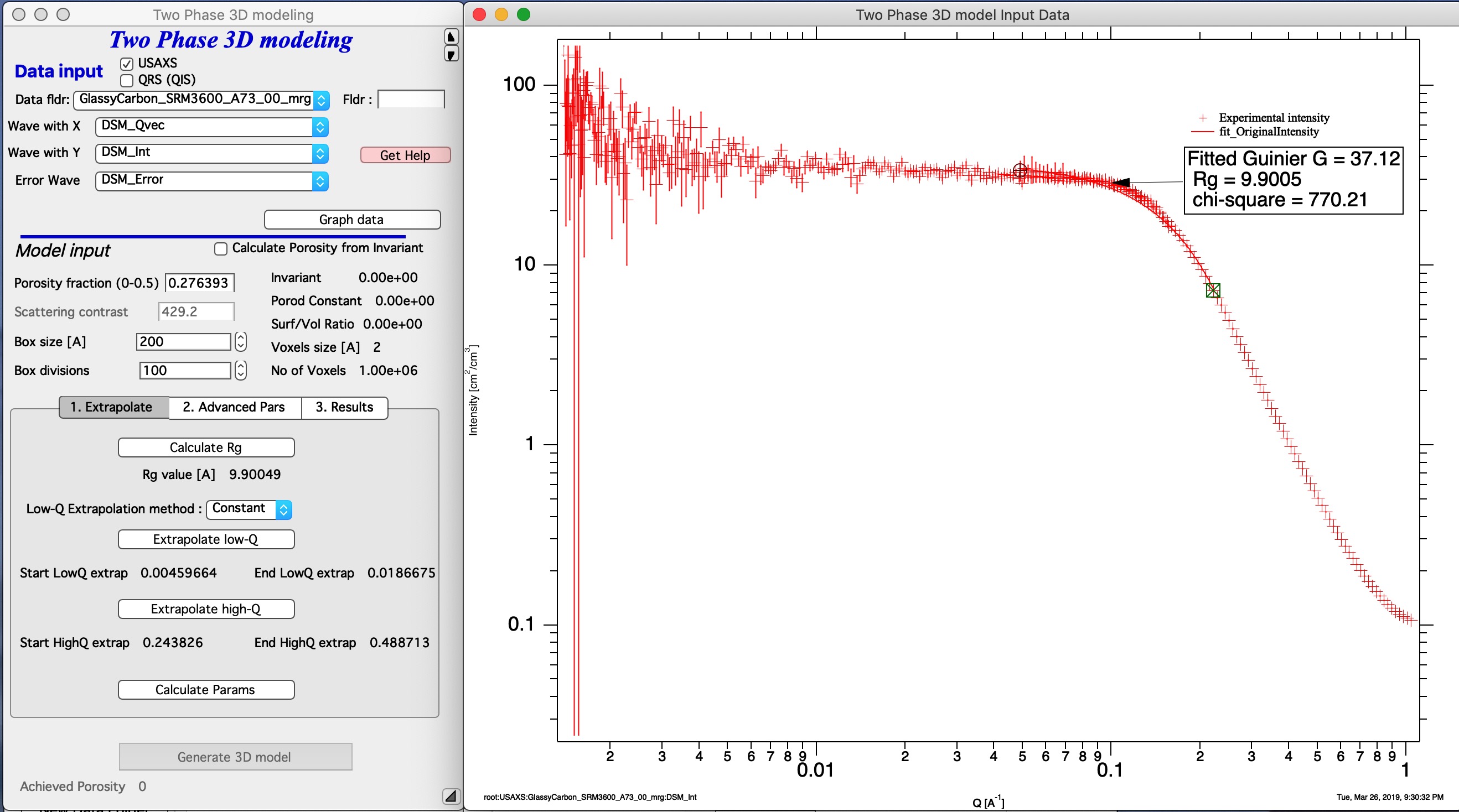
“Calculate Rg” — select the Guinier knee region with cursors and click this button to fit Rg. The result is used in the Advanced Parameters tab to set the maximum radius (10 × Rg).
Extrapolate to Q = 0 and Q = ∞:
Select the low-Q data range with cursors and click “Extrapolate low-Q”. Then select the high-Q range (where data follow Porod’s law, slope = −4) and click “Extrapolate high-Q” to extend the data to Q = 50.
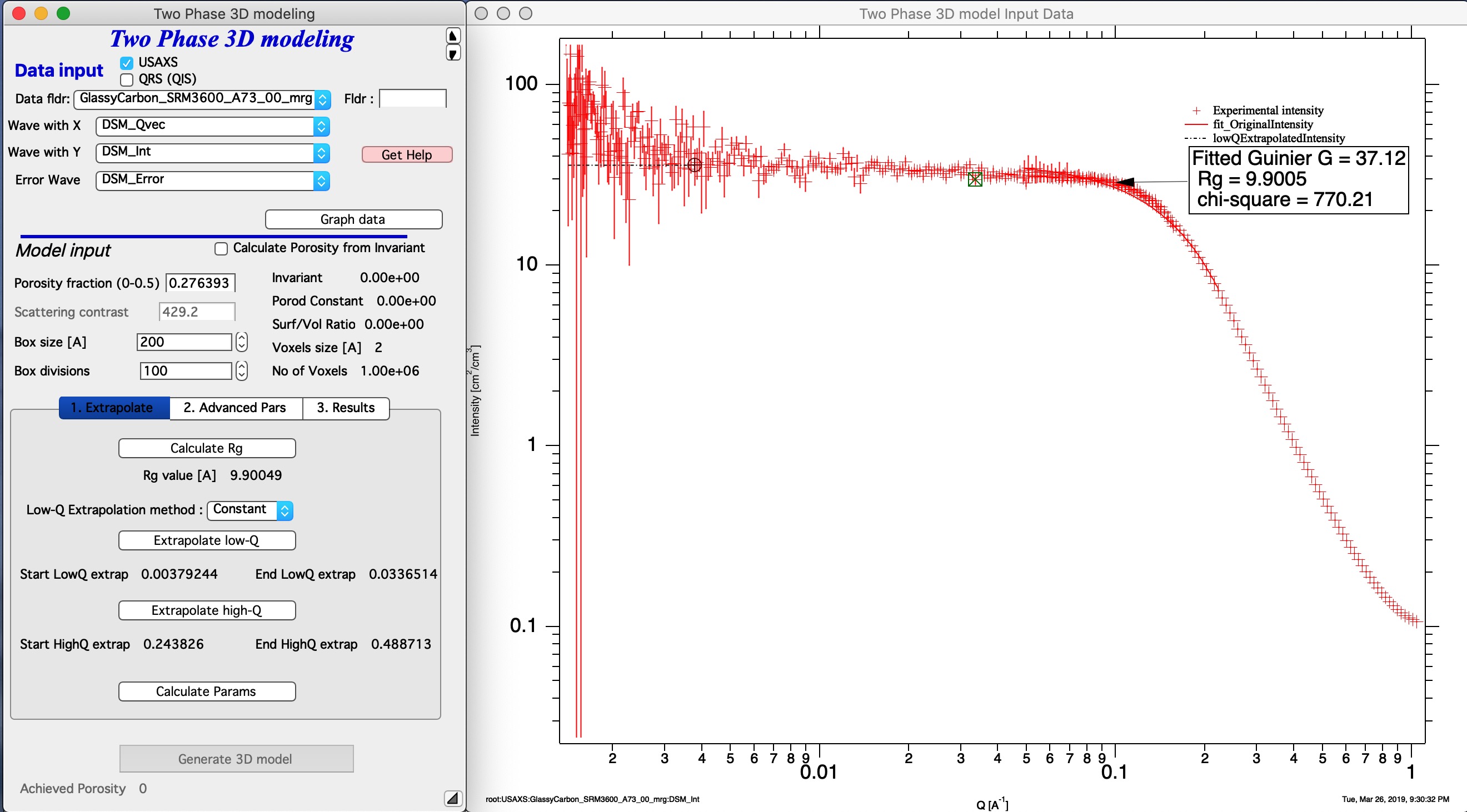

Click “Calculate Params” to compute all internal parameters, the invariant, and (if selected) the porosity. This step is required before generating the 3D model — the “Generate 3D model” button is disabled until it completes. An extrapolated intensity curve (from Q = 0 to Q = ∞) is added to the graph.
Note
The data should start with a flat (constant) intensity at low Q — no low-Q power-law slope is expected for a two-phase solid with smooth interfaces. At high Q the model assumes Porod’s law (slope = −4), which is appropriate for smooth solid/void interfaces.
Advanced parameters
Internal model parameters can be adjusted on the second tab.
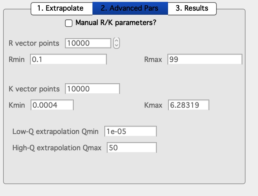
Enable “Manual R/K parameters?” to modify these values. These adjustments rarely produce significant improvements and should be used only with specific justification.
3D data generation
Click “Generate 3D model”. Generation time depends on the box divisions (approximately 45 seconds for typical settings). Most time is spent generating the Gaussian random fields. On completion, the back-calculated intensity from the Gaussian random field function is appended to the graph as the blue curve “TheoreticalIntensityDACF”.
The fit is typically good at low Q (extrapolation to Q = 0) and within approximately 1 decade in Q around Rg. With a resolution of 50–100 divisions, this is approximately the best achievable. Note that the modeled data are truncated and may show artifacts at the high-Q boundary of the fitted range due to numerical integration.
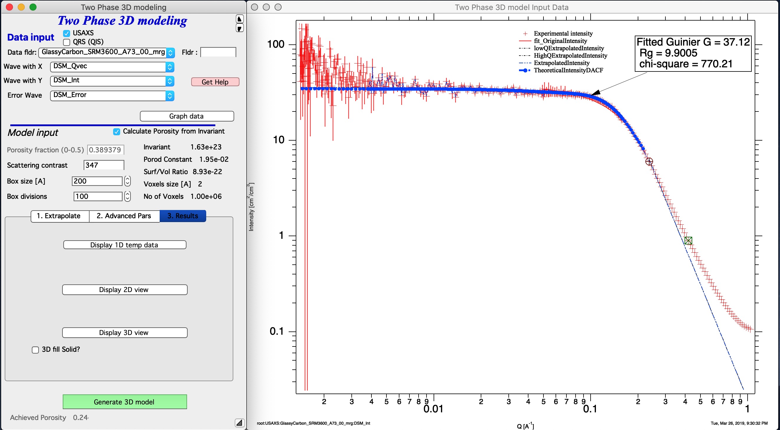
“Achieved Porosity” — calculated from the fraction of filled voxels in the generated model. This value will differ somewhat from the input porosity because a finite volume element is a statistical sample of infinite space; smaller box sizes show more variation.
Results display
The third tab contains visualization buttons.
“Display 1D temp data” — shows graphs for internal functions described in the SAXSMorph paper and manual. Informational only for most users.
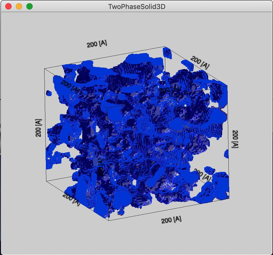
“Display 3D view” — generates a 3D Gizmo visualization of the Gaussian random fields. A checkbox selects whether the solid phase or the void phase is shown as filled.
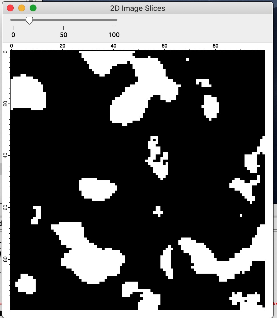
“Display 2D view” — generates a 2D cross-section through the 3D volume with a slider to step through slices. Since the field is isotropic, any cross-section is equally representative.
Model resolution considerations
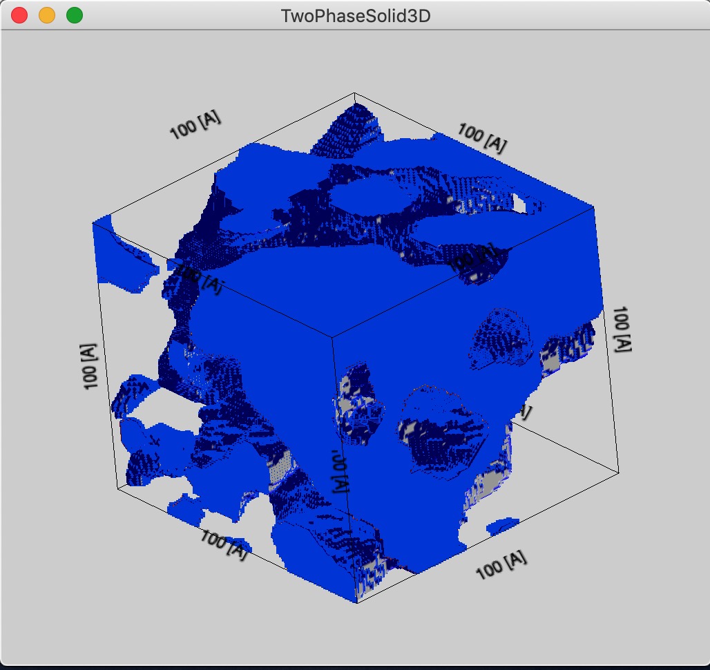
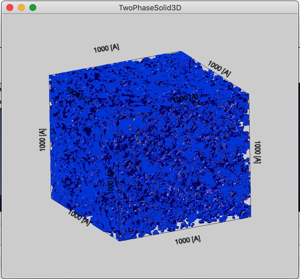
For a physically meaningful representation, the box size should be larger than the scale of the scatterers being modeled. The code sets Rmax (maximum modeled distance) to 10 × Rg, visible on the second tab. As a rule of thumb, the box size should be approximately 3 × Rmax.
Box size = 200 Å for a system with Rg ≈ 10 Å:
Box size = 100 Å — more structural detail visible but a less representative sample volume:
Box size = 1000 Å — highly representative but voxel size approaches Rg, making structural detail unresolvable:
Display 3D data
Displays 3D data using Igor Gizmo. This feature is not yet complete.
Import POV or PDB files
Imports POV files (generated by SAXSMorph) or PDB files (generated by ATSAS and other sources). This feature is not yet complete.