Guinier-Porod

Introduction

This model was developed by Boualem Hammouda (NIST) and published in:

“A new Guinier-Porod model,” J. Appl. Cryst. (2010), 43, 716–719.

In many ways it is similar to the Unified Fit model, but there are important differences. Reading the original papers on both theories before using this tool is strongly recommended.

Simplified description: Unified Fit vs Guinier-Porod

Unified Fit models scattering as a system of levels composed of Guinier and power-law (Porod) regions.

Guinier-Porod models scattering as a system of levels composed of Guinier and Porod (power-law) regions.

They are not equivalent.

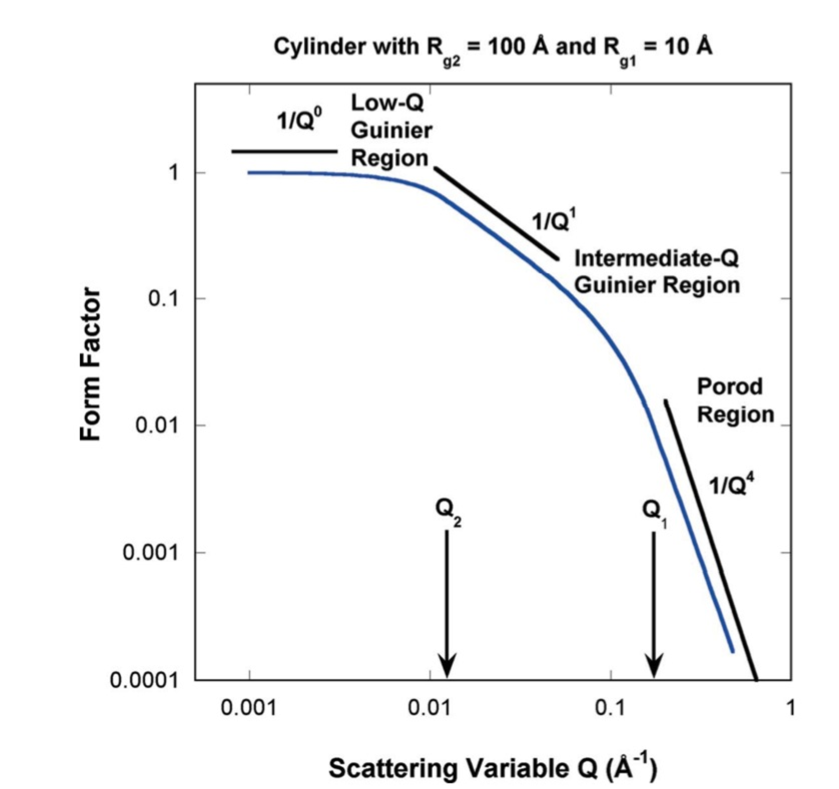
In the Guinier-Porod model, each level represents only one type of particulate system. For a particle with one characteristic dimension, there is one Guinier region and one power-law slope. For particles with two major dimensions (e.g., a rod), there are two Guinier regions and two power-law slopes. For three dimensions, the model uses two Guinier regions (the third is assumed too large to observe) and three power-law slopes. There is only one intensity scaling parameter per level (G).

See figures from the Hammouda manuscript for spheres (one dimension) and cylinders (two major dimensions):

One Guinier-Porod level can describe a particle with multiple main dimensions using 6 parameters. In contrast, representing the same system in Unified Fit requires multiple levels connected with RgCO. Although each Unified Fit level has fewer parameters than a Guinier-Porod level, complex systems in Unified Fit require many more levels — increasing the risk of reaching physically unreasonable solutions.

However, the Guinier-Porod model cannot describe systems that do not satisfy its assumptions: hierarchical fractal systems, polydisperse systems, etc. For example, Unified Fit can extract a log-normal size distribution from Guinier/Porod region mismatches — this is not possible in Guinier-Porod.

In summary: the Guinier-Porod model is superior for systems where its assumptions hold (approximately monodisperse, particulate systems). Unified Fit is more broadly applicable, though more challenging to use.

How to use the Guinier-Porod model

Parameter description:

Fitting with the Guinier-Porod model is more demanding than with Unified Fit, especially for USAXS slit-smeared data, which requires careful local fitting procedures.

Note

Local fits must be done in the order described on the panel; out-of-order fitting will produce incorrect results.

Main panel:

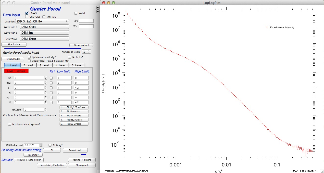
The top section contains standard data selection tools. This tool can be scripted using the Scripting tool. Select the data naming system and dataset, then click “Graph data”.

---

Controls above the Level tabs:

“Number of levels” — selects how many levels to use. Build levels incrementally: fit level 1 first, then add level 2, and so on. More than 3 levels are rarely needed.

“Graph model” — forces recalculation of the model with current parameters.

“Update automatically” — recalculates after every parameter change. Recommended for fast computers.

“Display Local Fits” — shows local Guinier and power-law fits. These are computed only when local fits are run.

“No limits” — removes all fitting bounds. Often useful because some parameters (like G) can span many decades.

The tabbed area contains GP model parameter inputs; background is below the tabs.

Buttons:

“Fit” — least-squares fit of checked parameters within the cursor range.

“Revert back” — restores parameters to their pre-fit values.

“Fix limits” — resets fitting limits around current parameter values. Use this if a “reached fitting limit” message appears.

“Results →Data Folder” — saves results to the source data folder as GuinierPorodFitIntensity_Y and GuinierPorodFitQvector_Y, where Y is an order number. Optionally exports per-level intensity as GuinierPorodIntLevelX_Y / GuinierPorodQvecLevelX_Y.

“Results →Graphs” — adds parameter tags to the graph.

“Clean graph” — removes tags from the graph.

“Uncertainty evaluation” — same as in Unified Fit and Modeling II.

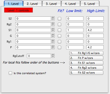
Model Parameters (tabbed area):

Parameters are ordered from top (low-Q effects) to bottom (high-Q effects): S2, Rg2, S1, G, Rg1, P. Local fitting must follow the numbered button order, not the visual top-to-bottom order.

The additional parameter RgCutOff terminates level scattering at a size threshold, for hierarchical structures (see Unified Fit documentation). For non-spherical particles, the appropriate value of RgCutOff can be complex — consult the theory before using it.

“Is this correlated system?” — adds an Interferences structure factor, same as in Unified Fit. Using this for non-spherical particles is generally not physically justified.

Fitting procedure

Example with data fitted by a two-level Unified Fit model:

Step-by-step procedure:

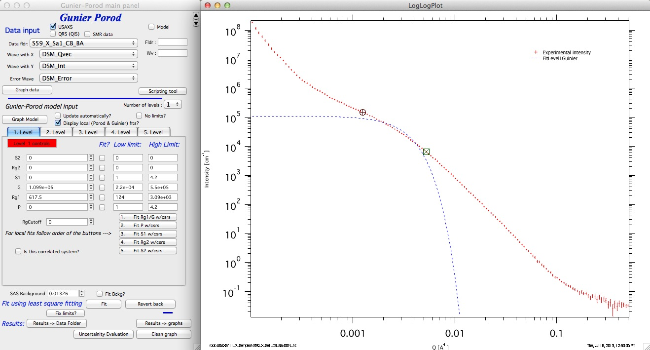
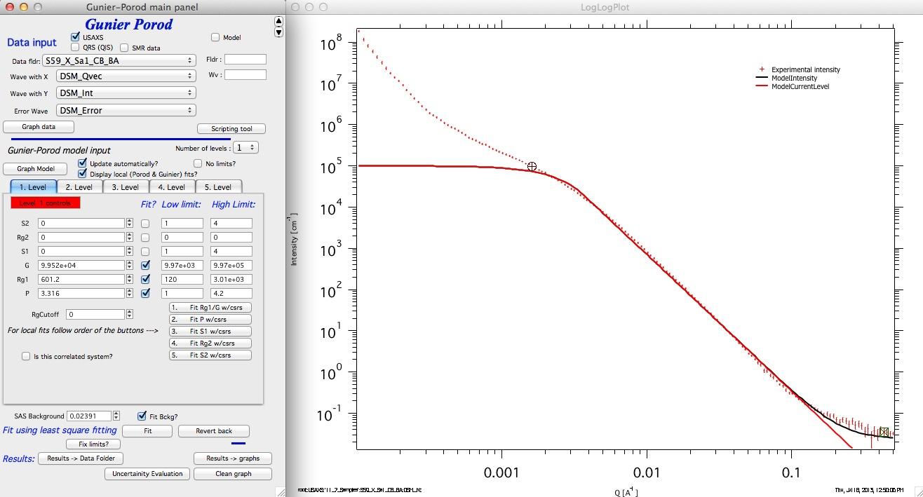
1. Set “Number of levels” to 1. Place cursors over the Guinier region and click “1. Fit Rg1/G w/csrs”. Do not adjust checkboxes, starting values, or limits — these are handled automatically.

   

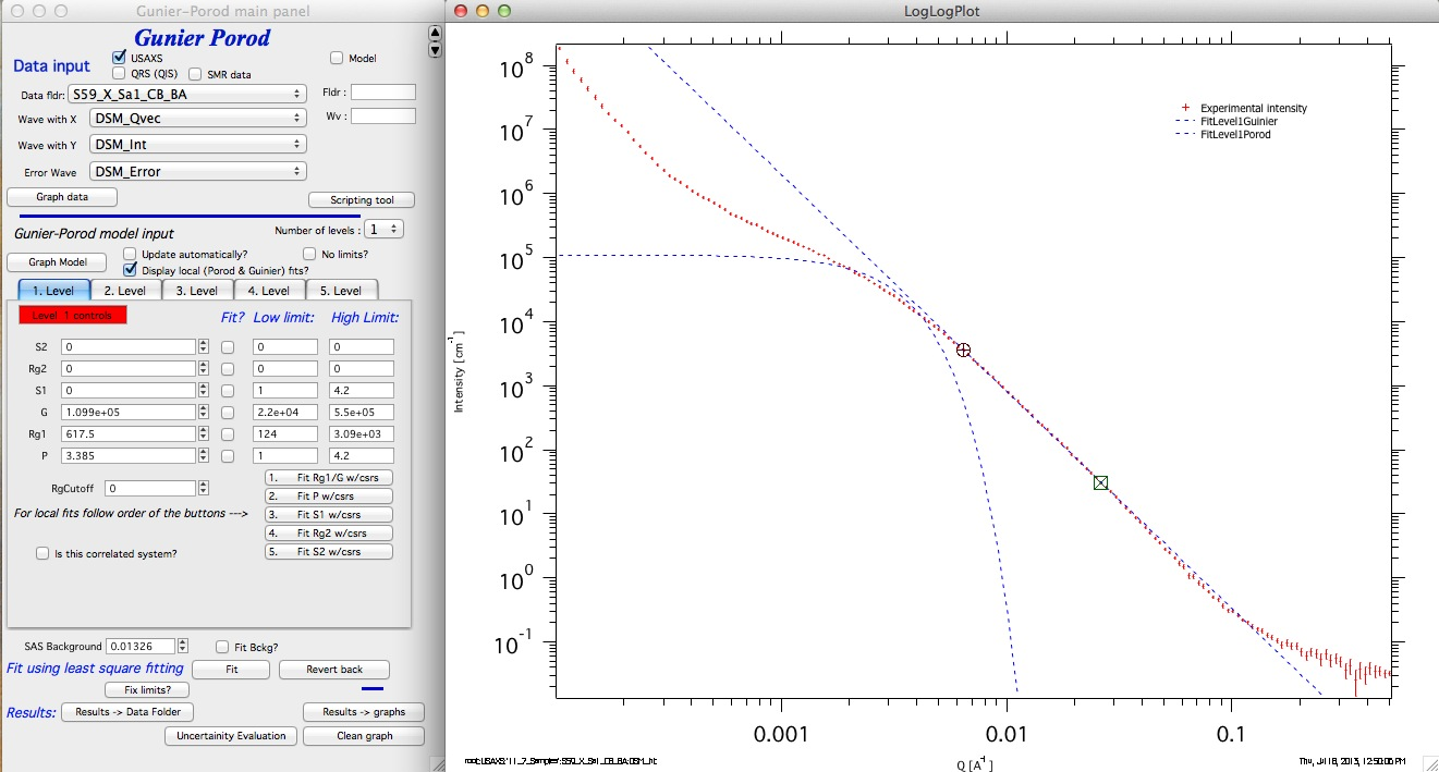
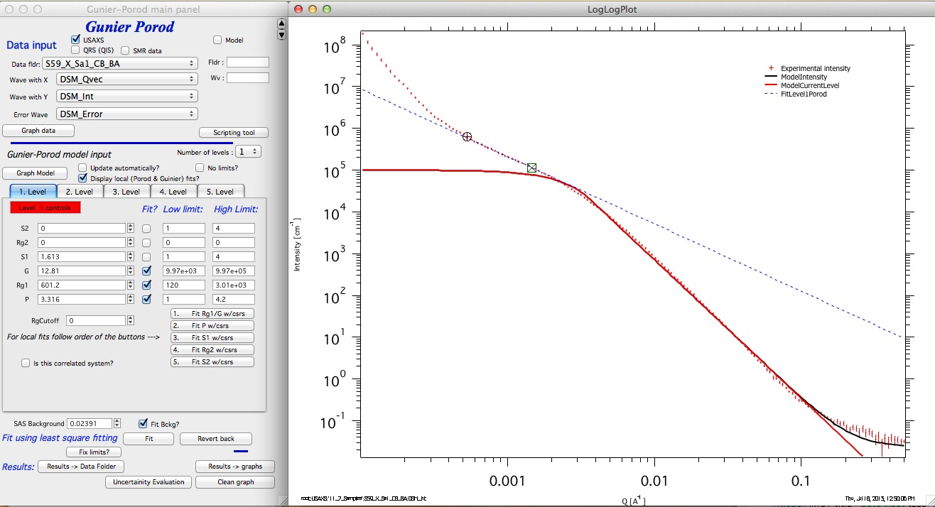
2. Move cursors to the high-Q power-law region and click “2. Fit P w/csrs”:

   

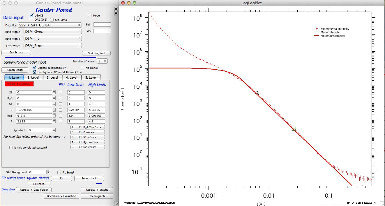
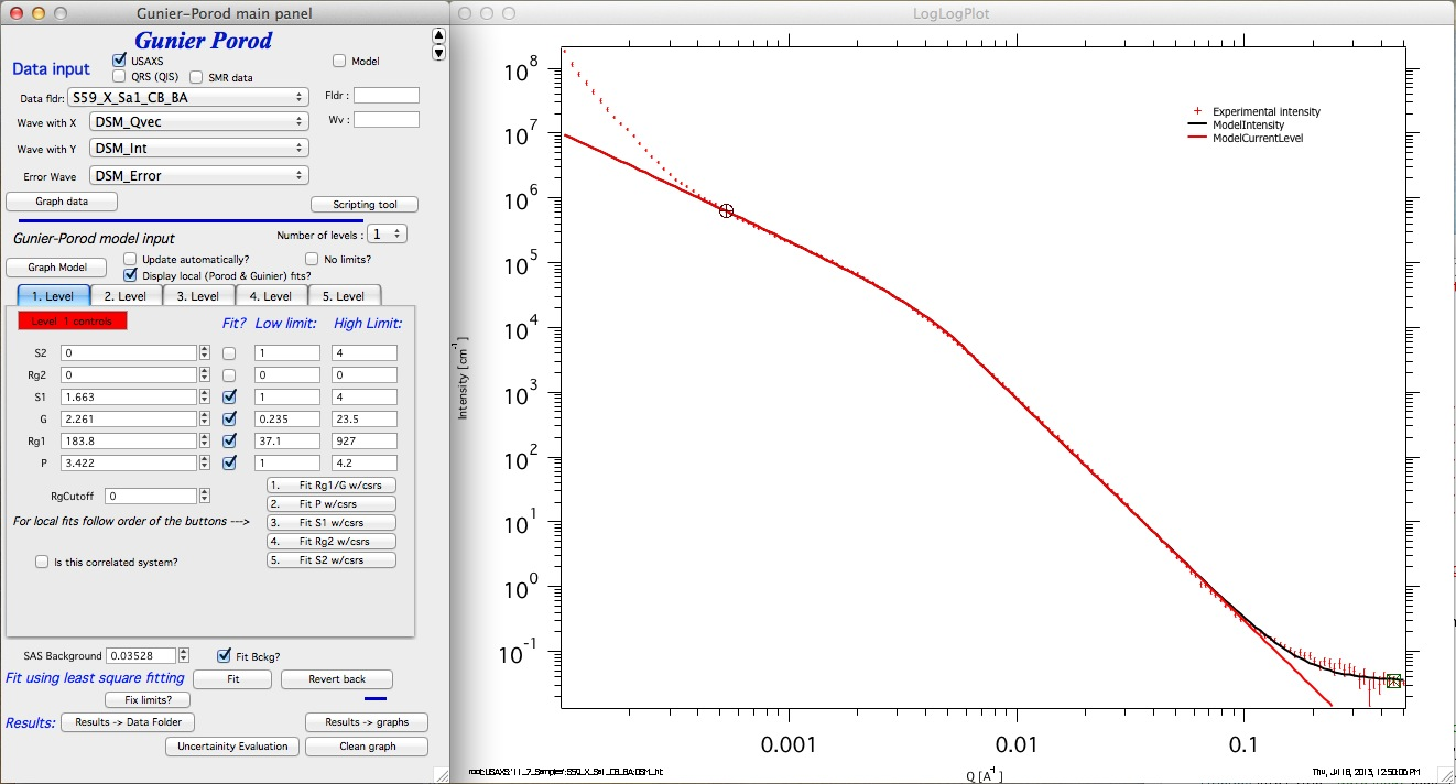
3. Click “Graph Model” (or enable “Update automatically”) to display the current GP model:

   

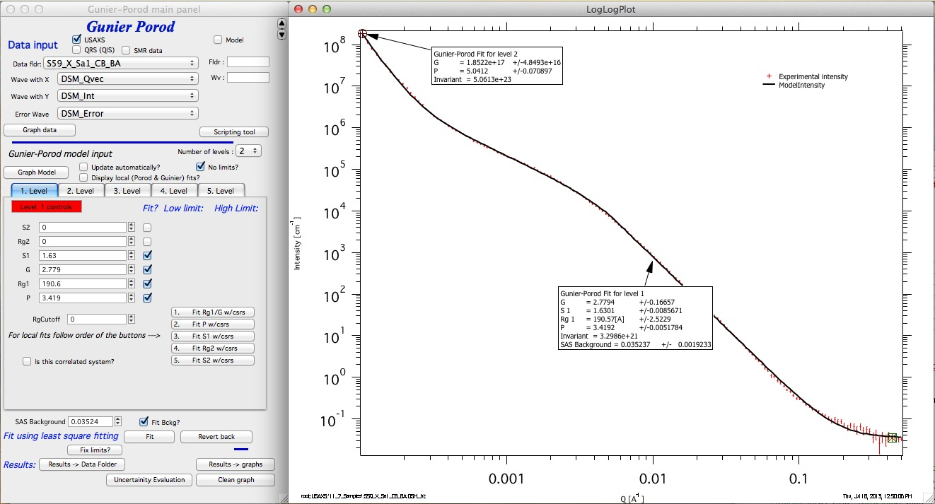
4. Add a background estimate (read from the high-Q region), select the full data range, check “Fit?” for G, P, Rg1, and background, and click “Fit”:

   

   If fitting limits are reached, click “Fix limits?” and retry, or enable “No limits?” — this typically works without issue for GP fits.

5. Add the S1 slope: place cursors on the low-Q power-law region and click “3. Fit S1 w/csrs”:

   

   A slope of ~1.6 suggests a particle between a rod (S1 = 1) and a disk (S1 = 2). Select data from cursor A position to high Q, check “Fit?” for S1, and fit the full range:

   

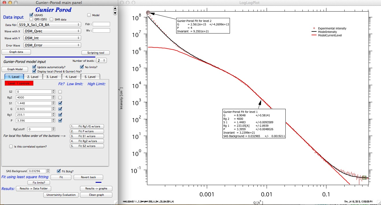
6. The low-Q slope suggests another structural level. Add Level 2 via the “Number of levels” popup. Set Rg1 = 1×10⁶ (this triggers internal handling for a pure power-law level where the Guinier knee is not visible). Click “2. Fit P w/csrs”:

   

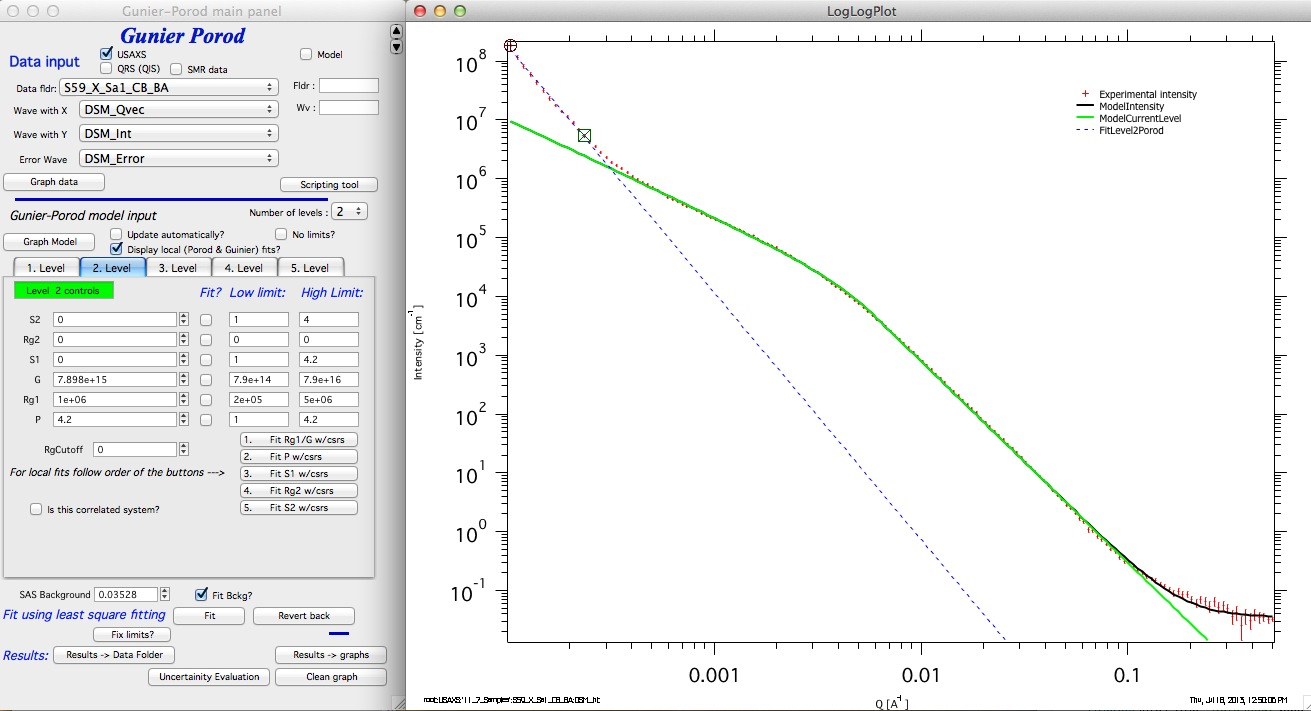
   For Level 2, fit G and P (Rg1 stays fixed at 1×10⁶). For Level 1, fit P, Rg1, G, S1, and background. Disabling limits is safe here:

   

   This is the best model justified by the scattering data alone.

7. If additional physical constraints are known (e.g., power-law slope > 4 is physically unusual at low Q), they can be imposed to make the model more physically meaningful:

   

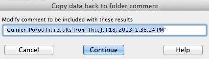
8. Save results using “Results→Data Folder” and provide a meaningful title:

   

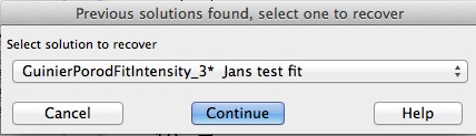
   Results waves (intensity and Q vector) are saved with all GP parameters in the wave note. These can be exported, plotted, and mined with the Data Mining tool. When a dataset with saved results is reloaded, the tool offers to restore the stored parameters: