Powder diffraction (WAXS) fitting

Purpose and description

This tool provides simple analysis of powder diffraction data. Its scope is limited to:

1. Displaying WAXS data — one dataset at a time. Multiple datasets can be displayed using the Plotting tool.

2. Appending diffraction line sets (PDF2/4 d-hkl-Intensity data) to the displayed data. Several PDF cards calculated from model assumptions are included in the Irena distribution and additional cards can be imported from JCPDS XML format. A previous interface to LaueGo was removed in version 2.62 due to compatibility instability; contact the developer if this capability is needed.

3. Fitting diffraction peaks — one dataset at a time or as a sequence, using WaveMetrics’ Multi Peak Fitting 2.0 (MPF2). Only Gaussian and Lorentzian peak shapes are fully supported for result recording and downstream processing.

Data requirements

The tool accepts qrs or USAXS data (slit smearing is not supported). The QRS naming convention handles:

• Q [Å^-1] — Intensity — Uncertainty (qrs)

• d [Å] — Intensity — Uncertainty (drs)

• 2θ [degrees] — Intensity — Uncertainty (trs)

All input types are converted to 2θ [degrees] — Intensity — Uncertainty for plotting and analysis.

Basic GUI and operations

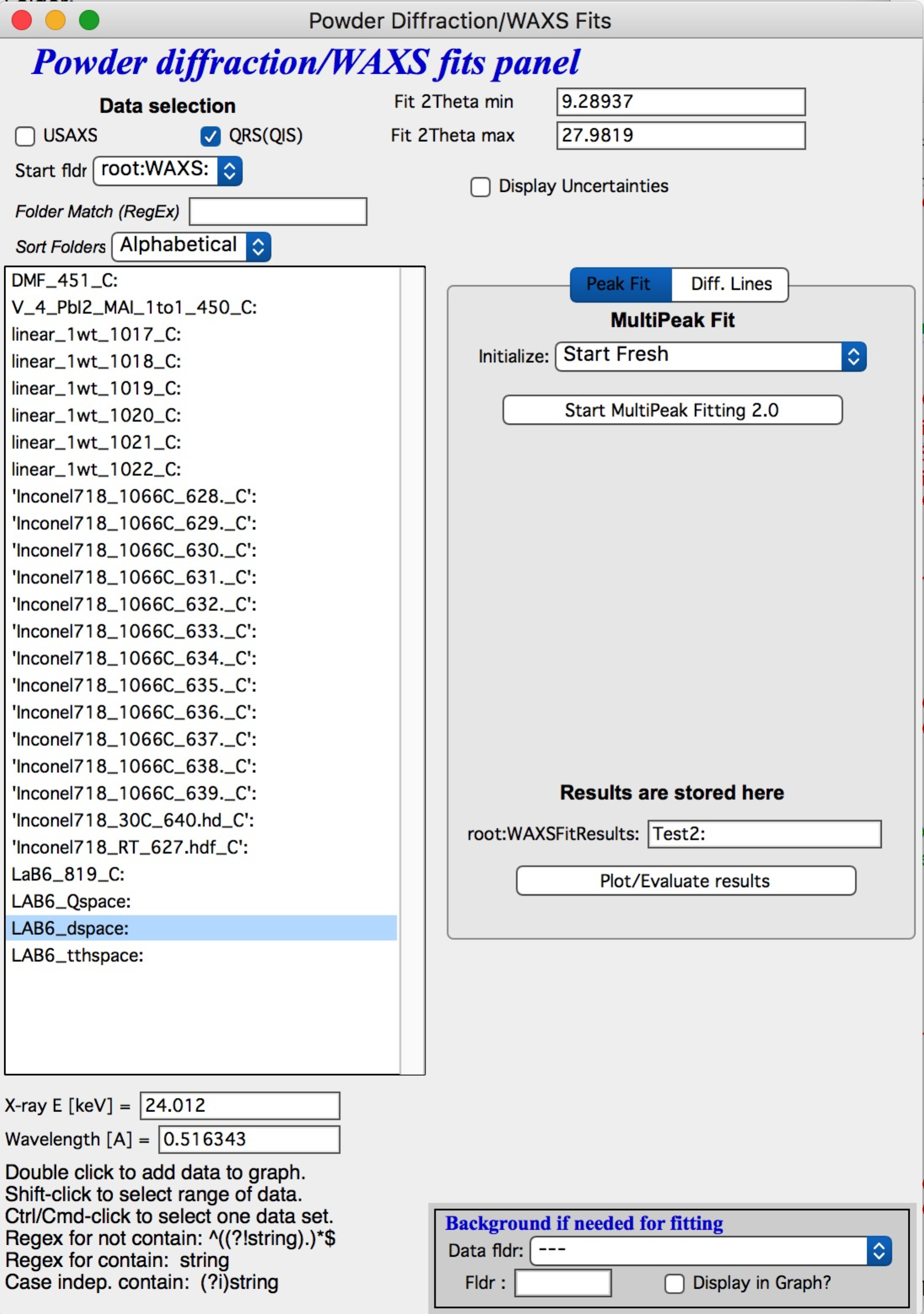
Select “Powder Diffraction fitting = WAXS” from the SAS menu.

In the GUI: select the data type (most likely QRS), the folder containing your data, optionally filter folders using regular expressions, and select the sort order. Sort order is important for sequential in-situ experiments, both for fitting and for obtaining correctly ordered results when the data are later “mined” for parameter changes.

Double-clicking a dataset opens the graph. If the wave note contains energy or wavelength information, it is displayed. An approximately correct wavelength is required; for two-theta data, it must be exact.

Set the fitting range using cursors or by entering 2θ min/max values manually. Background selection (from a measured empty exposure) is used only if it is a significant contribution and will be applied during peak fitting.

The graph

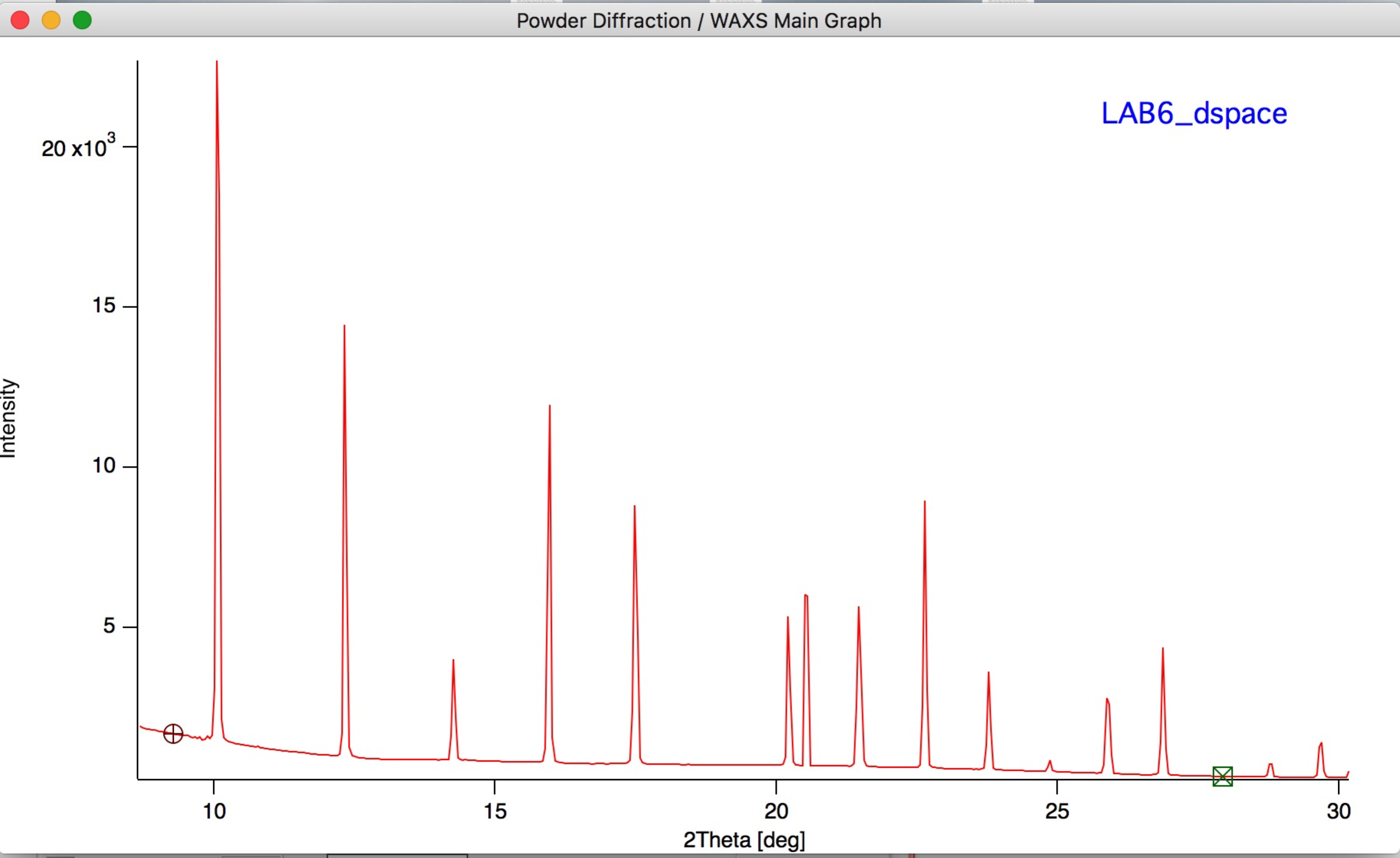
Data are displayed as Intensity vs 2θ (degrees).

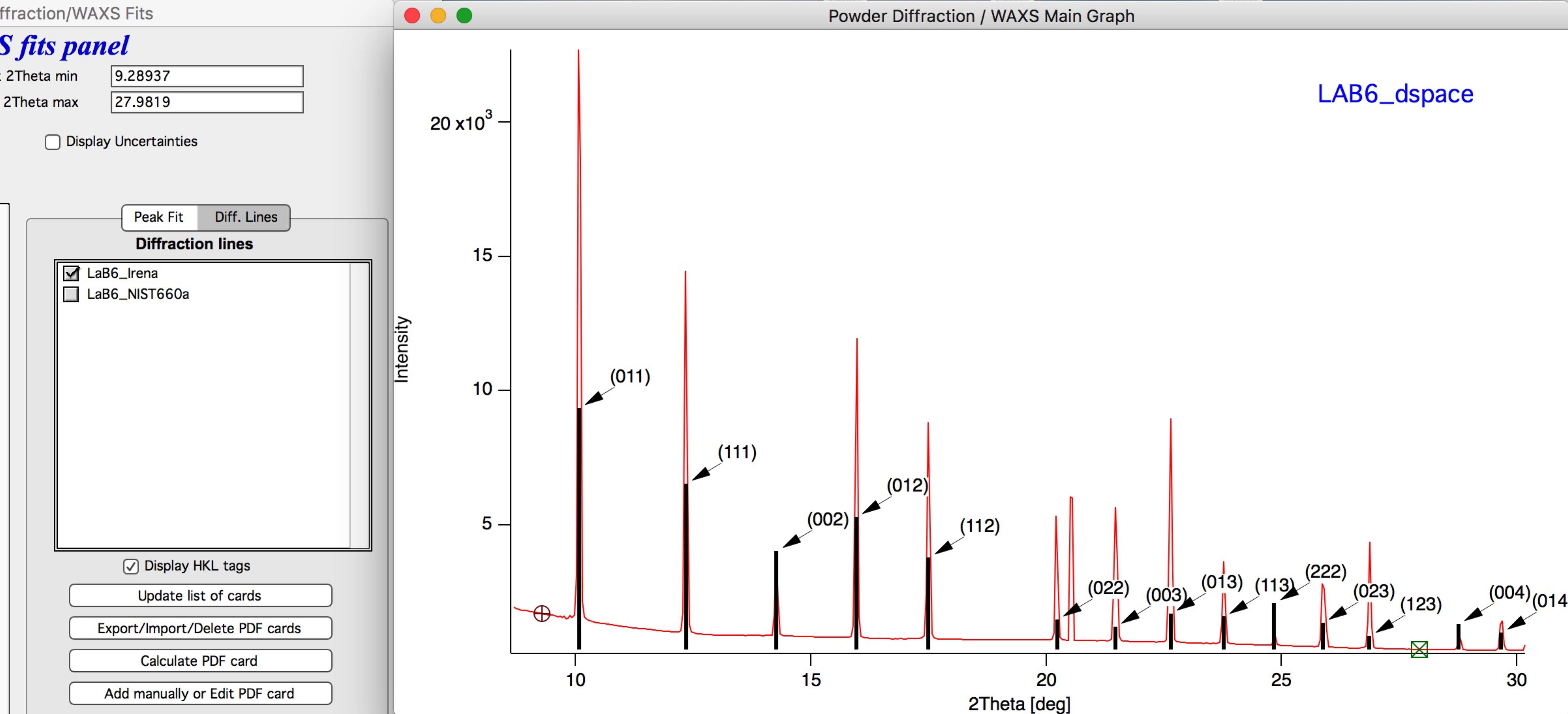
Adding diffraction lines (PDF2/4-type)

For phase identification, JCPDS PDF data or the free American Mineralogist Crystal Structure Database (AMS, http://rruff.geo.arizona.edu/AMS/amcsd.php) can be used. Irena cannot connect directly to these databases, but supports importing cards manually.

Click the “Diff. lines” tab on the right side of the panel. Several calculated cards are distributed with Irena.

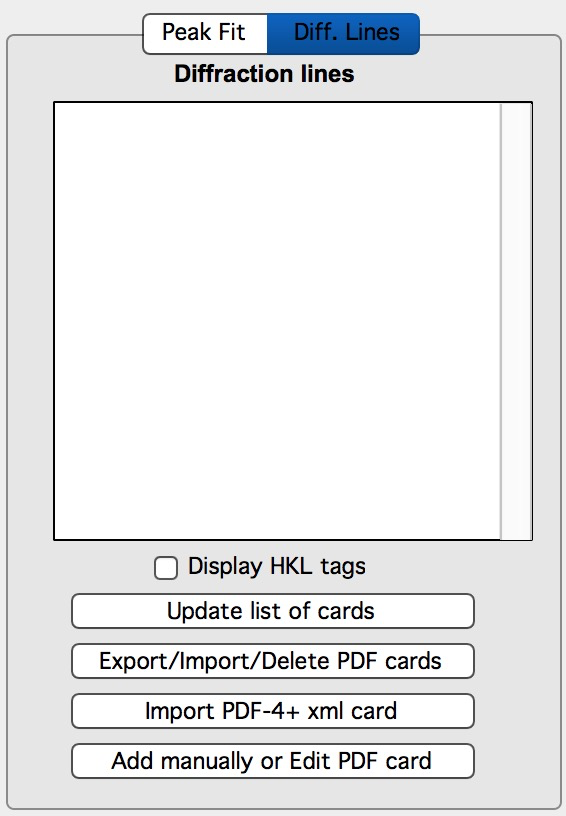
Options for adding diffraction lines:

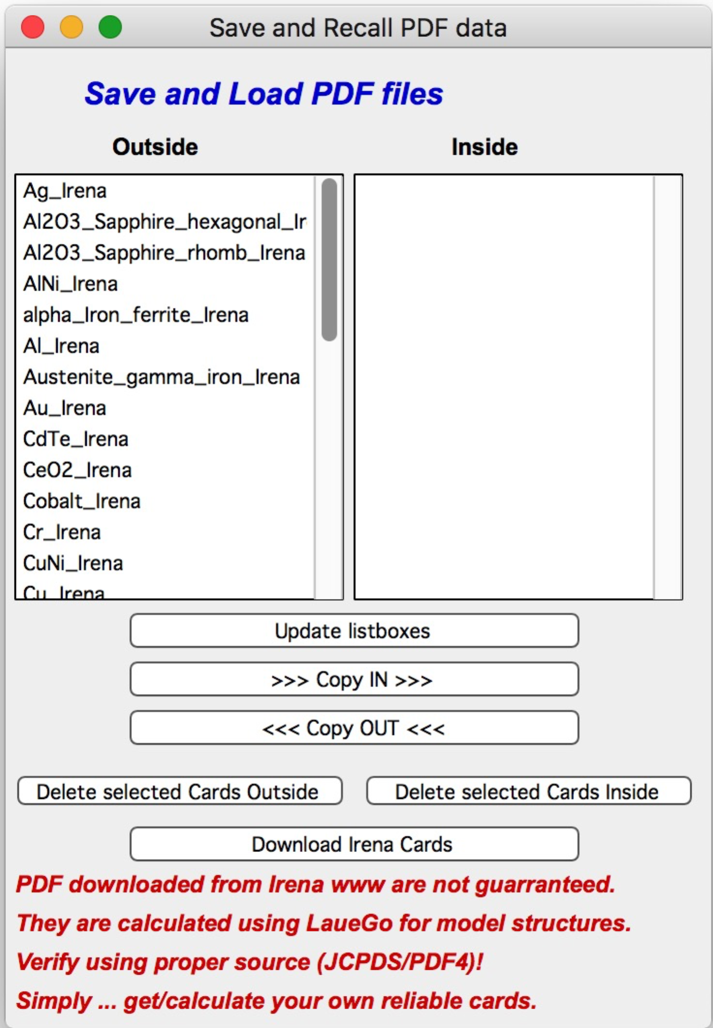
1. Import from the Irena distribution — click “Export/Import/Delete PDF cards” to open a card management GUI. Cards outside Igor (distributed with Irena) can be copied in; user-created cards can be copied out for storage. Refresh the list after any external changes.

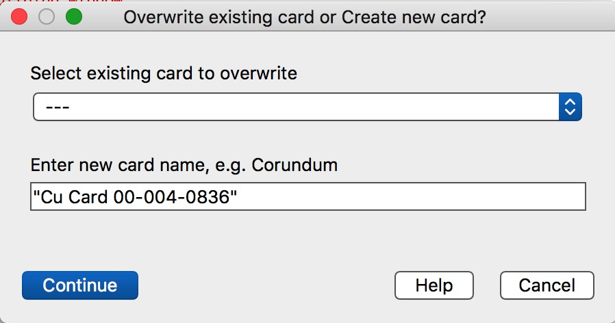
2. Import PDF-4+ XML cards — click the import button, locate the XML card file, and select whether to overwrite an existing card or create a new one:

   

3. Import AMS txt cards — same procedure as JCPDS, but point the file selector to AMS_DATA.txt files from the AMS database. Download “diffraction data” (not crystal structures).

4. Add data manually — creates an empty table for manual entry or paste from another application. At minimum, d-spacing and intensity are required; HKL values are helpful. Two-theta values are calculated automatically from the current wavelength.

After adding cards, enable “Display HKL tags” to annotate each peak with its HKL indices:

Right-click a card name in the listbox to change its display color.

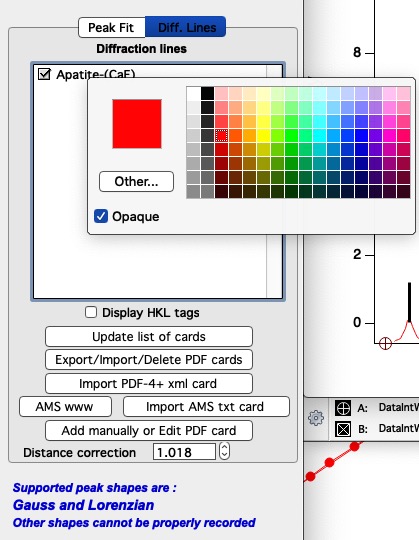
“Distance correction” (from version 2.692, May 2020) — A correction factor for tweaking stick positions when the detector distance calibration is slightly off. The default is 1.0. This shifts the angular positions of the diffraction sticks only (not the d-spacing values in the tables) and affects only JCPDS/AMS cards. The value resets to 1.0 when the WAXS tool is reopened.

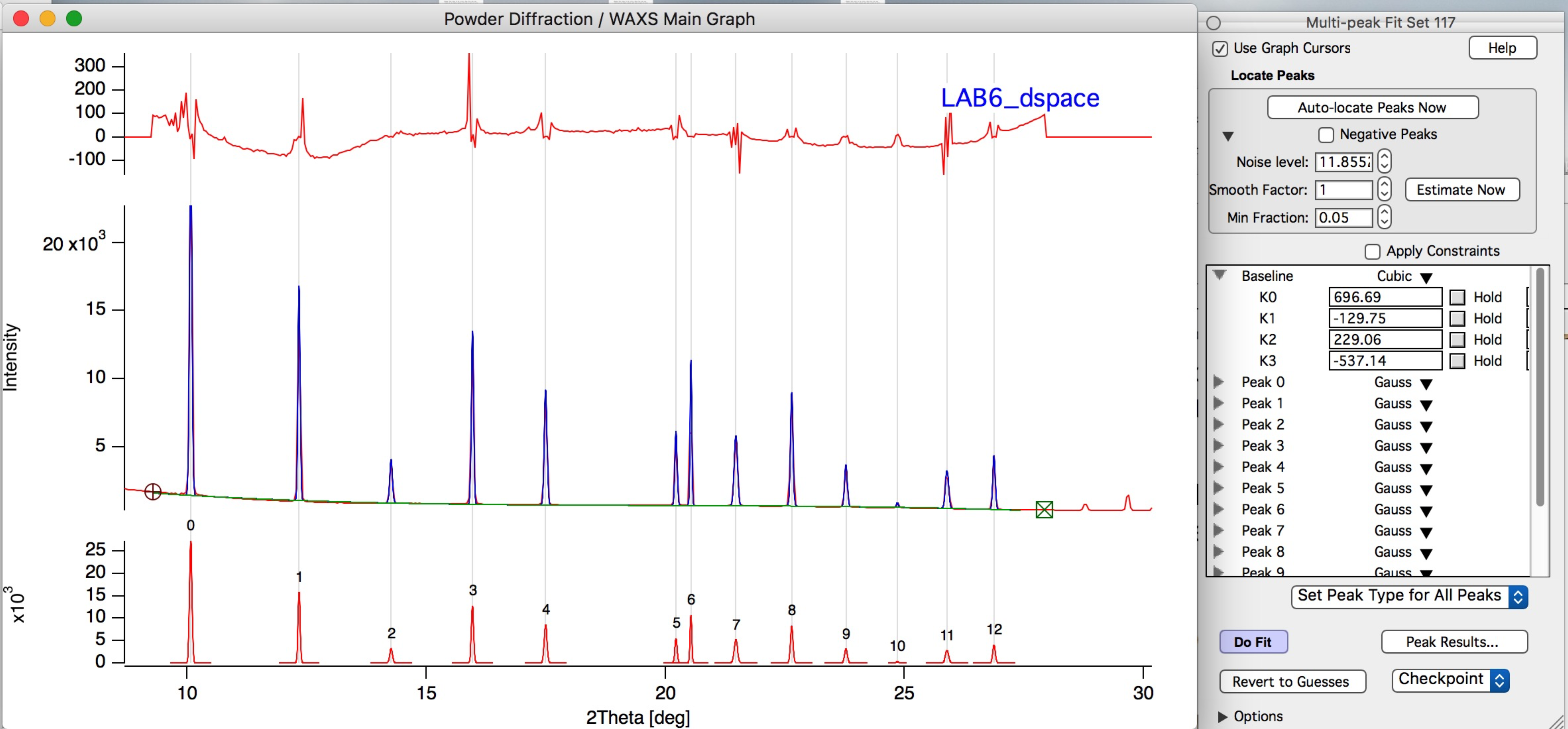
Peak fitting

The “Peak Fit” tab contains peak fitting tools using WaveMetrics’ Multi Peak Fitting 2.0 (MPF2). The MPF2 demo experiment at

File → Example Experiments → Curve Fitting → Multi-peak Fit 2 demo

provides a thorough introduction to MPF2 and is strongly recommended before using this feature.

Start MPF2 by clicking “Start Multipeak Fitting 2.0” — the data graph must be open. An error is displayed if no graph is available. MPF2 saves its state in run folders; when closing the panel, an optional comment can be added to identify the run later.

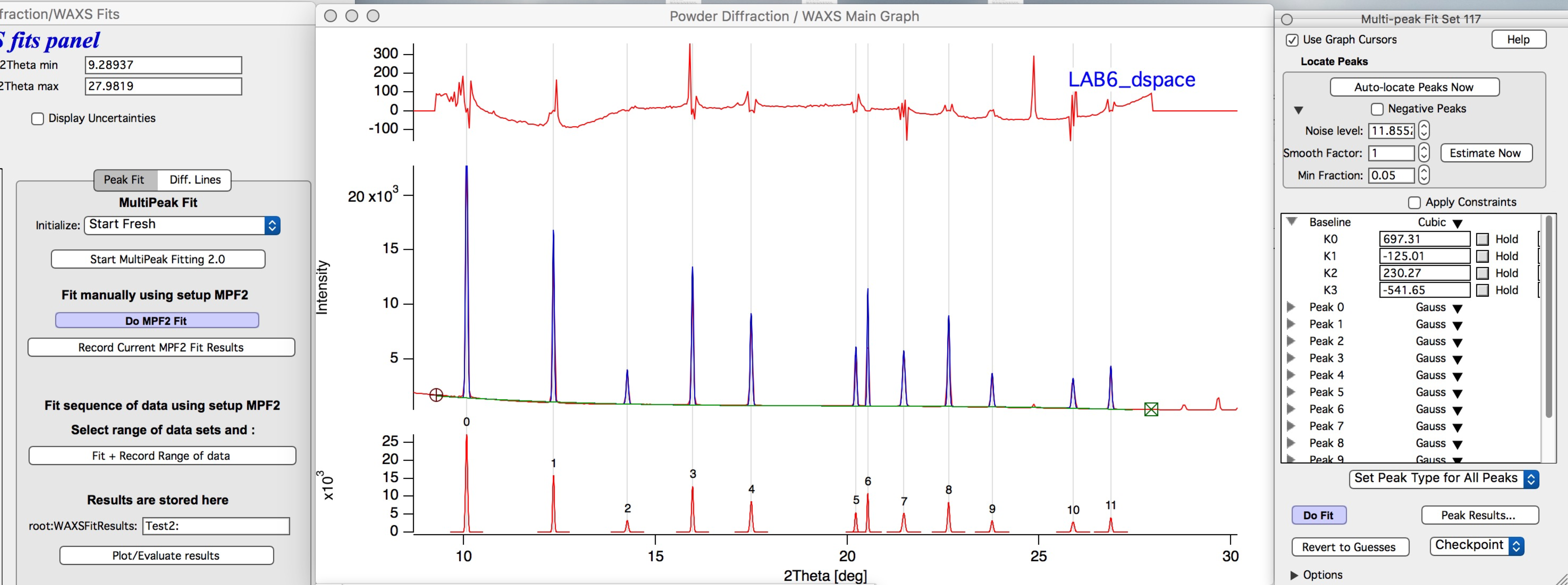
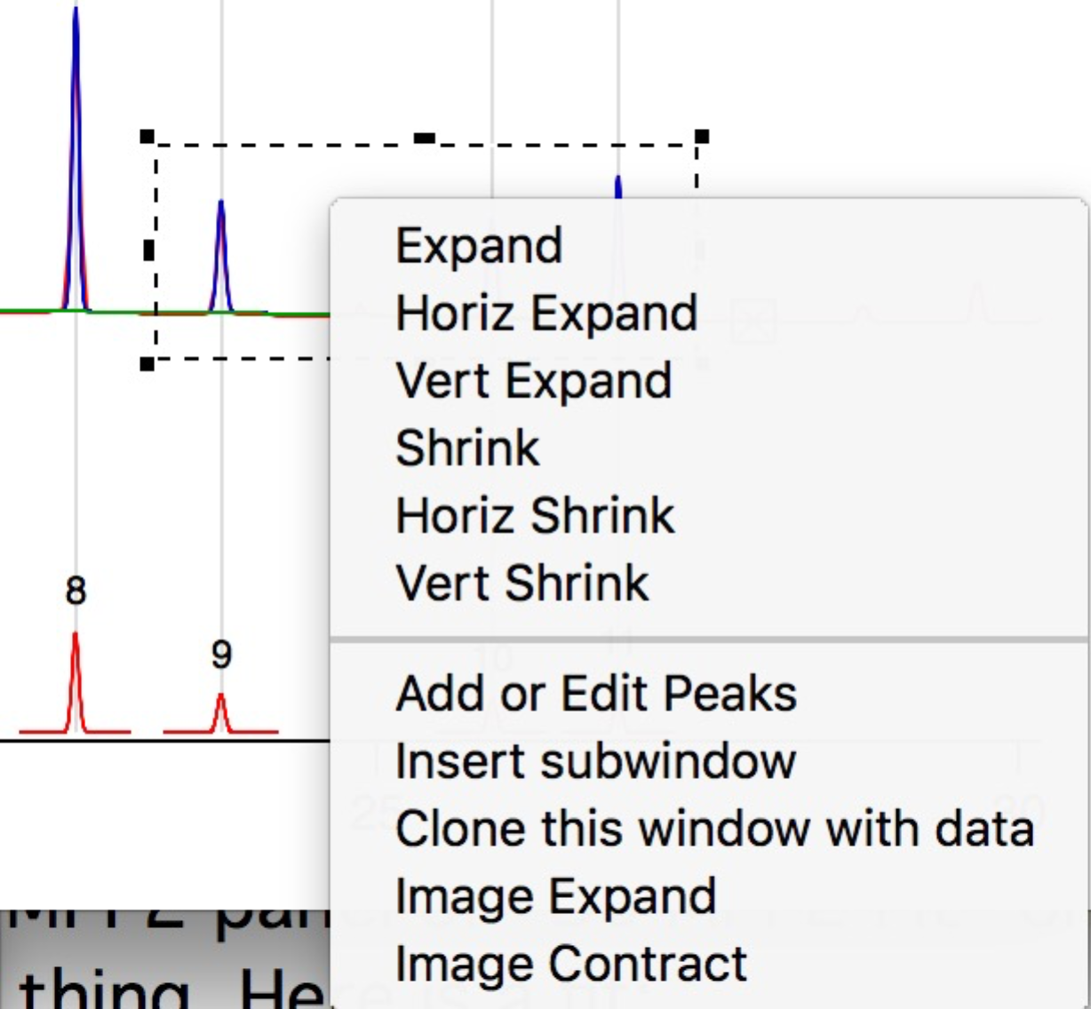
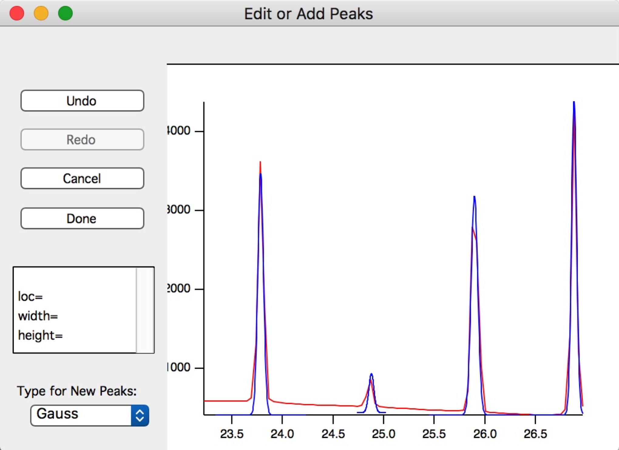
Set up MPF2: select the data range with cursors, run “Autolocate”, zoom in as needed, and add or edit peaks by right-clicking within a marquee selection.

Baseline function options in MPF2 (standard options plus two added by Irena):

• Polynomial — up to 10th order; hold unused coefficients at 0.

• Measured background + constant — scales a measured background image by a fitted “transmission” factor and adds a constant flat background. If no background data are loaded, this reduces to a simple constant baseline.

Fitting can be run with the “Do Fit” button on the MPF2 panel or the “Do MPF2 Fit” button on the Powder Diffraction panel — both are equivalent.

When satisfied with the fit, click “Record Current MPF2 Fit results”. Results are saved to a folder under root:WAXSFitResults: with the name specified in the panel (cleaned up to be a valid Igor folder name). Each sample gets its own subfolder containing results tables and individual peak profiles. Saving results for the same sample overwrites the existing folder.

Results tables are displayed automatically after saving.

To plot or evaluate results across multiple samples, click “Plot/Evaluate results” to open a dedicated panel. Selecting a specific peak and folder set plots that peak’s profile across all available results:

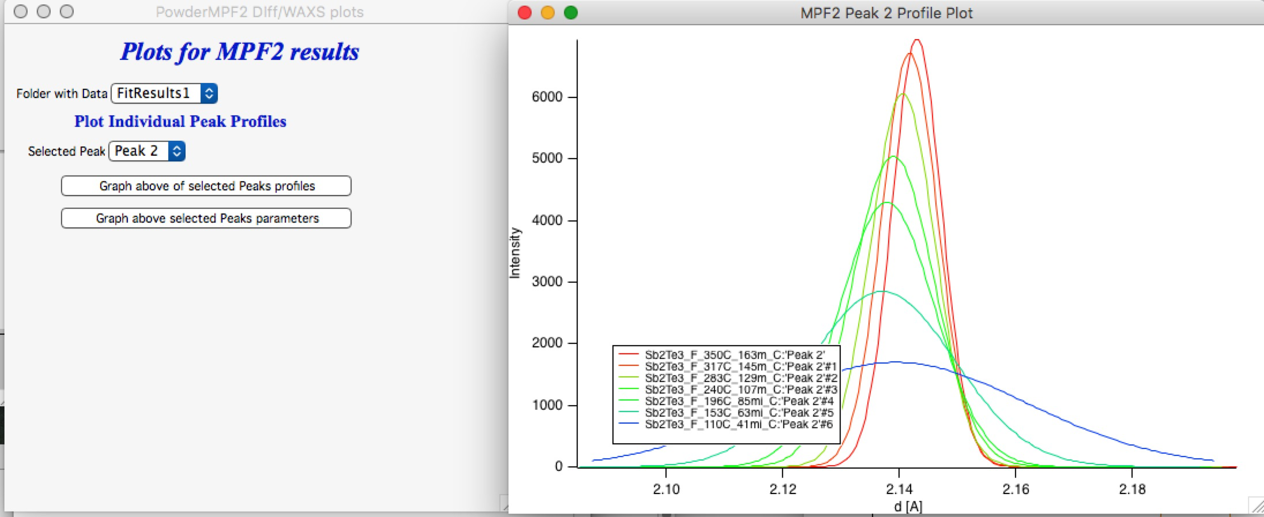
Example: peak profile (Intensity vs d) for Peak 2 from a temperature series.

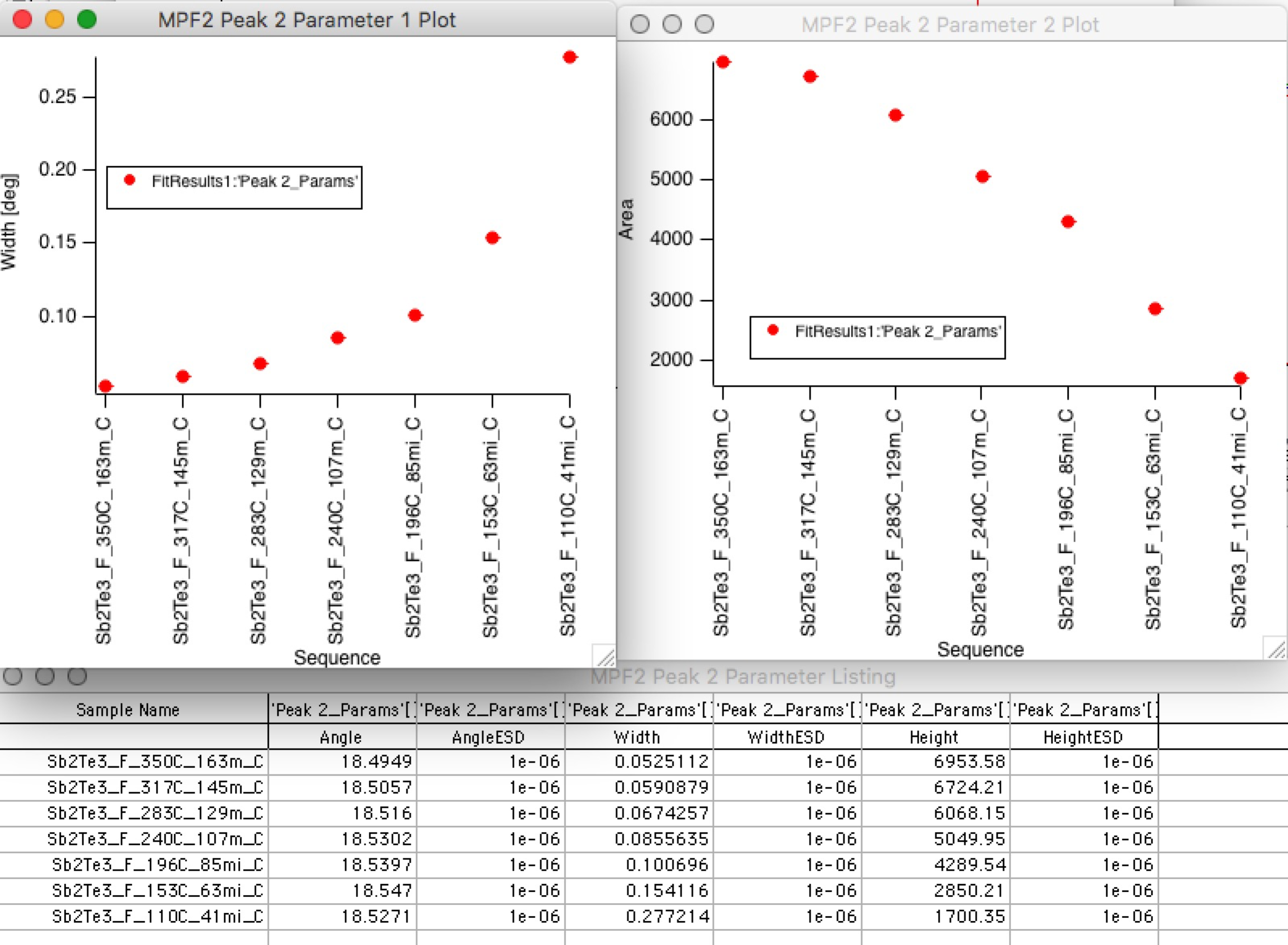
Example: peak parameters (position, width, area) from the same series, plotted against sample index.