Fractal model

This model was developed by Andrew J. Allen (NIST, Andrew.allen@nist.gov). It allows combining up to two volume (mass) fractals and two surface fractals in a manner similar to the Unified model. The parameters have the advantage of being more directly fractal-related than those from Unified Fit. A short PDF description is included in the distribution and served as the basis for this implementation. The Igor code is a port of Andrew’s original Fortran code and has been verified to produce identical results.

Please cite:

G. Gadikota, F. Zhang, A. J. Allen, “Towards understanding the microstructural and structural changes in natural hierarchical materials for energy recovery: In-operando multi-scale X-ray scattering characterization of Na- and Ca-montmorillonite on heating to 1150 °C,” Fuel, 196, 195–209 (2017). DOI: 10.1016/j.fuel.2017.01.092

Important points for proper analysis

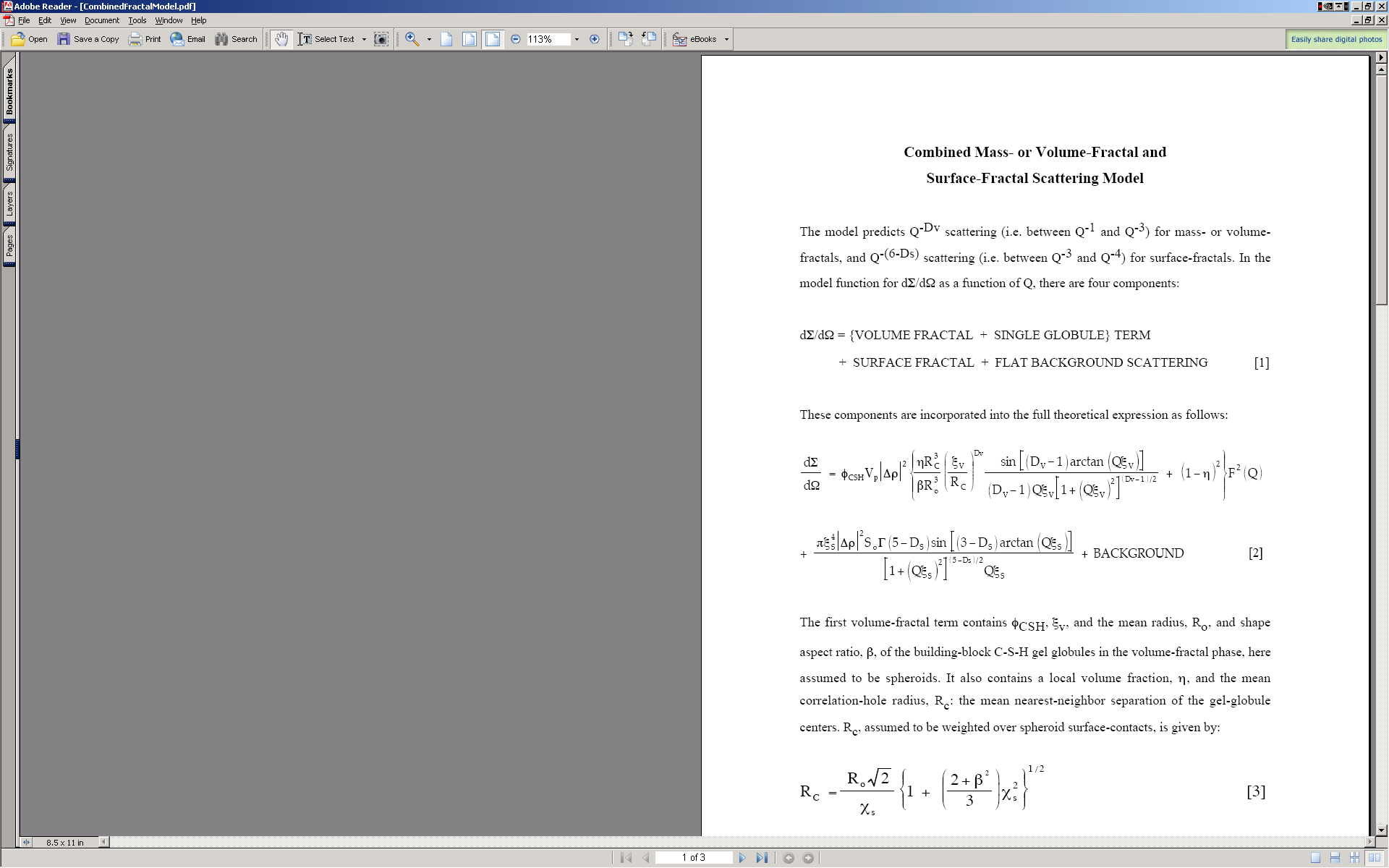
• Make realistic initial parameter estimates. Fix the flat background to an effective subtracted value initially (a small amount of refinement in the final fit is acceptable). Porod law fitting in an appropriate Q range is useful for this — it also provides a total surface area S_t from which the rough surface-fractal surface area S_sf can be subtracted to yield the volume-fractal surface area S_vf.

• The η parameter should generally be fixed at approximately 0.5 initially, with limited refinement in the final fit.

Key challenge: For a single volume-fractal and single surface-fractal component plus background, there are in principle 9 fitting parameters. However, each distinct region of the scattering curve with approximately one curvature typically requires only 3 parameters for convergence in that region. A minimum of 3 distinct regions in the data is needed to fit all parameters reliably.

A recommended fitting approach: start with reasonable initial parameters and achieve a semi-acceptable fit to the whole curve, then focus on individual Q regions to refine each parameter set while fixing the others. Iterate until all parameters are well constrained.

Model description

Use

Note

USAXS data used with this model must be desmeared (DSM). The tool does not recognize slit-smeared data.

Real fractal data are not included in the distribution, but the included example data are sufficient for demonstrating GUI functionality.

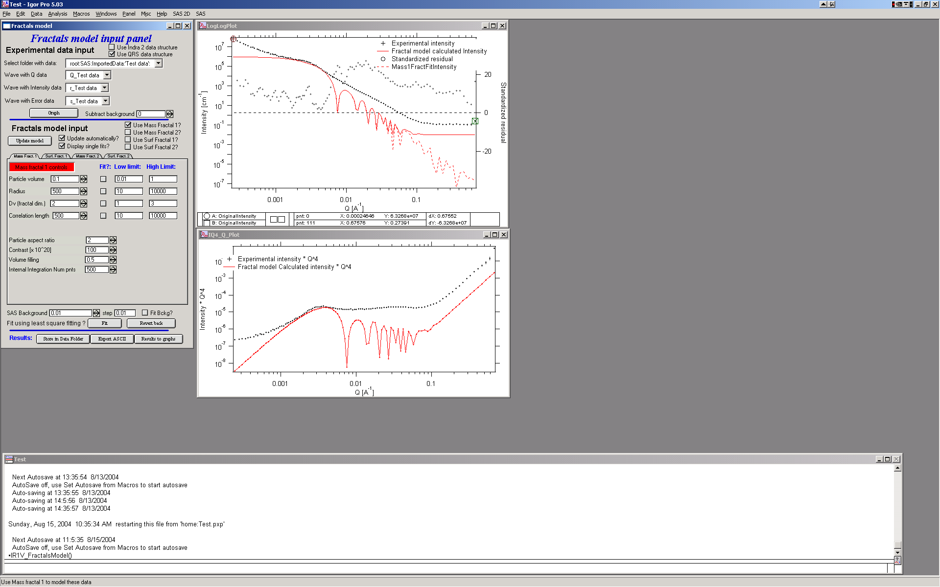
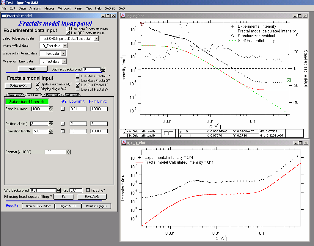
Start the tool from the SAS menu under “Fractal model”. Select “Use QRS data structure” and pick the available dataset, then click “Graph” to create the graphs.

The “Subtract background” variable next to the data selection allows subtracting a known fixed large background before fitting. The “SAS Background” parameter at the bottom is a similar term but is refined during fitting.

Select “Use mass fractal 1” and configure checkboxes as shown:

Any combination of the two mass fractals and two surface fractals can be used.

Mass fractal parameters

Particle volume — volume of a single primary particle.

Particle radius — radius of a primary particle.

Dv — volume-fractal dimension.

Correlation length — mean nearest-neighbor separation between particles.

Particle aspect ratio (beta) — primary particles are spheroids with dimensions R × R × β·R.

• β = 1: spheres (most common)

• β > 1: elongated spheroids (prolate, “cigars”)

• β < 1: flattened spheroids (oblate, “disks”)

The code uses monodisperse form factors (sphere or spheroid), which produce Bessel-function oscillations at high Q. These oscillations are rarely physically realistic. Unless a surface fractal is present at high Q to obscure them, the model may appear unrealistic in that range.

Use UF Particle Form Factor (from Irena version 2.70) — uses the Unified Fit approximate sphere form factor, which is free of Bessel-function oscillations. Aspect ratio β is fixed at 1 when this option is selected.

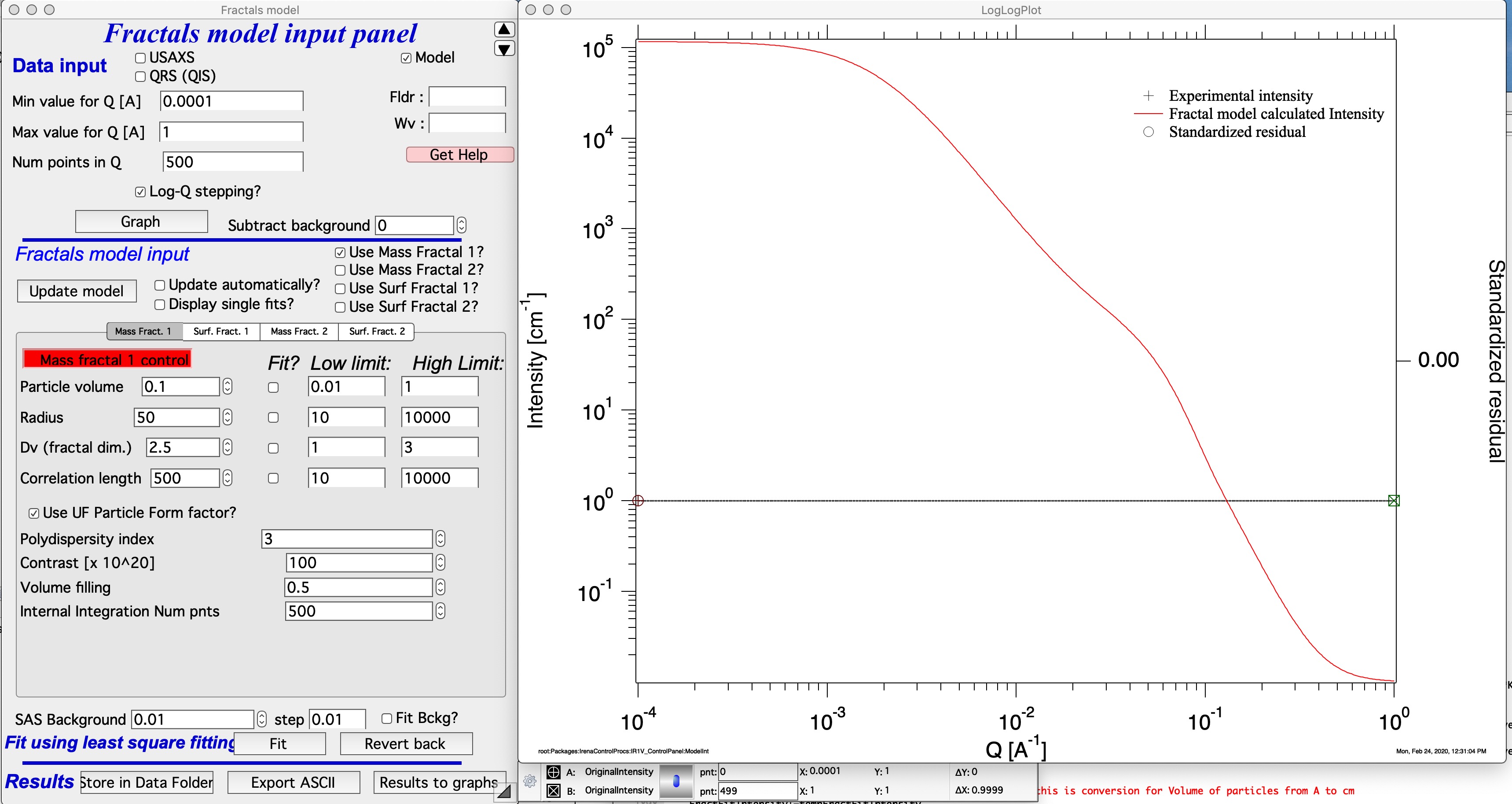
Polydispersity index (PDI) — available when “Use UF Particle Form Factor” is selected. Represents the size distribution of primary particles.

• PDI = 1: monodisperse

• PDI = 3: Porod region fully merges with the Guinier region

• PDI = 5–10: highly polydisperse

Typical systems require PDI between 1 and 5.

Contrast — scattering contrast.

Volume filling — volume fraction of the fractal phase.

Internal integration Num pnts — number of points in the numerical orientational-average integral. Too few points (especially at high aspect ratios) cause artifacts; too many increase calculation time significantly.

Recommended approach: start with a lower number of points to find good initial parameters, then increase to verify convergence for the final fit. If the result does not change when the number of points is doubled, the chosen value is adequate. Keep volume filling between approximately 0.4 and 0.6.

Surface fractal parameters

Select “Use Surf Fractal 1” (and deselect the mass fractal if testing independently):

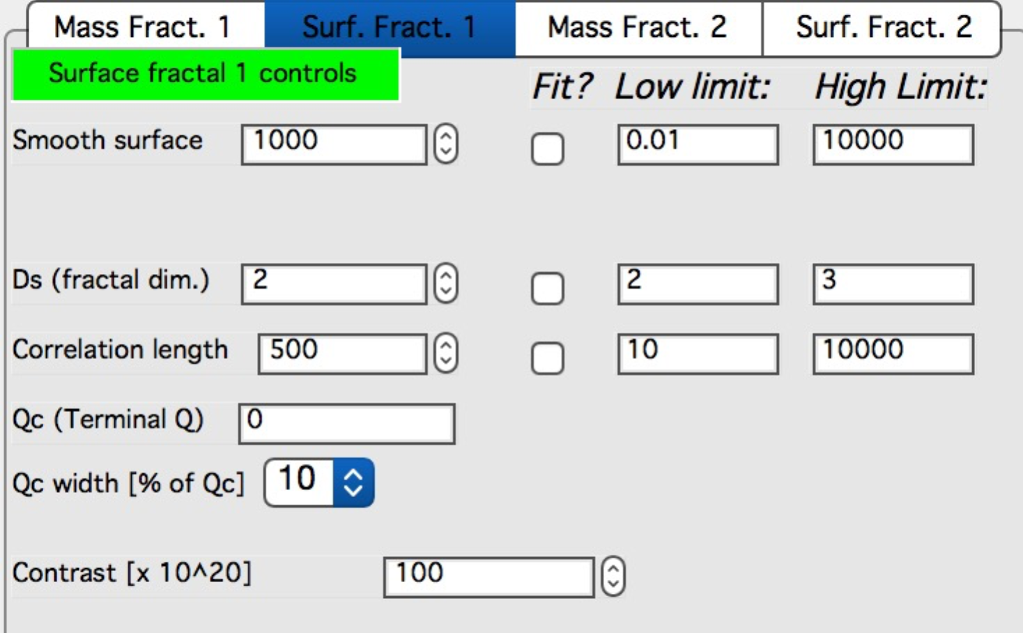
Smooth surface — upper limit of smooth surface scattering (see model description above).

Ds — surface-fractal dimension.

Correlation length — correlation length as defined in the theory.

Qc (Terminal Q) — Q value at which scattering transitions from the surface fractal regime to smooth-surface Porod scattering (I ∝ Q^-4).

Qc width [% of Qc] — smoothing parameter for the turnover at Q_c. Typical value: 10% (options: 5, 10, 15, 20, 25%).

Contrast — scattering contrast.

The fitting approach is the same as for Unified Fit: first find good starting conditions manually, then use cursors to select the appropriate Q range and apply least-squares fitting with the desired parameters free.