Simple fits tool
This tool performs rapid simple fits on many datasets. Configure the Q range and fitting conditions on one or two datasets and then run the tool on all selected datasets. With a suitable Q range and model, you quickly obtain a table or graph of results for the entire set.
Implemented models:
Guinier
Porod
Sphere
Spheroid
Guinier Rod
Guinier Sheet
Invariant
1D Correlation
Power Law
Selecting data
Familiarity with the data selection tools simplifies use of this panel. In the Data selection area, define the data to analyze. Full details are available in Multi Data selection. The tool accepts three data types: USAXS, QRS (SAXS or WAXS), and Irena results. SAXS/WAXS data that do not come from the APS USAXS instrument use the QRS naming system; use USAXS only for APS USAXS data. For Irena results, the two applicable types are Volume and Number size distribution outputs.
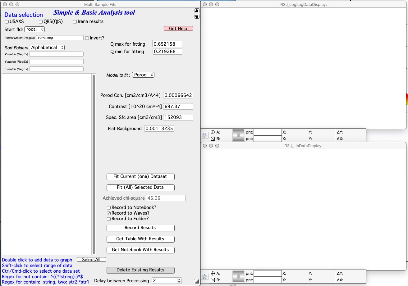
Select Start fldr (e.g., root:SAXS:) and a data type using Folder
Match (e.g., sub).
Add data by double-clicking in the folder list. Data are always added to the top graph as log-Intensity vs log-Q. For some models (Guinier, Porod, etc.), the lower graph shows a linearization plot.
Select the Q range for the desired model and click “Fit Current (One) Dataset”. Results appear alongside the graph:
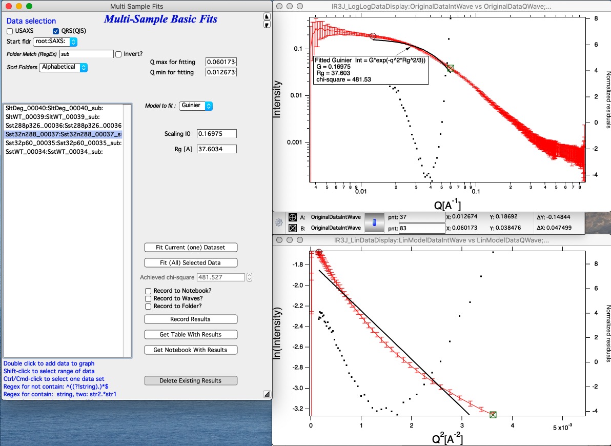
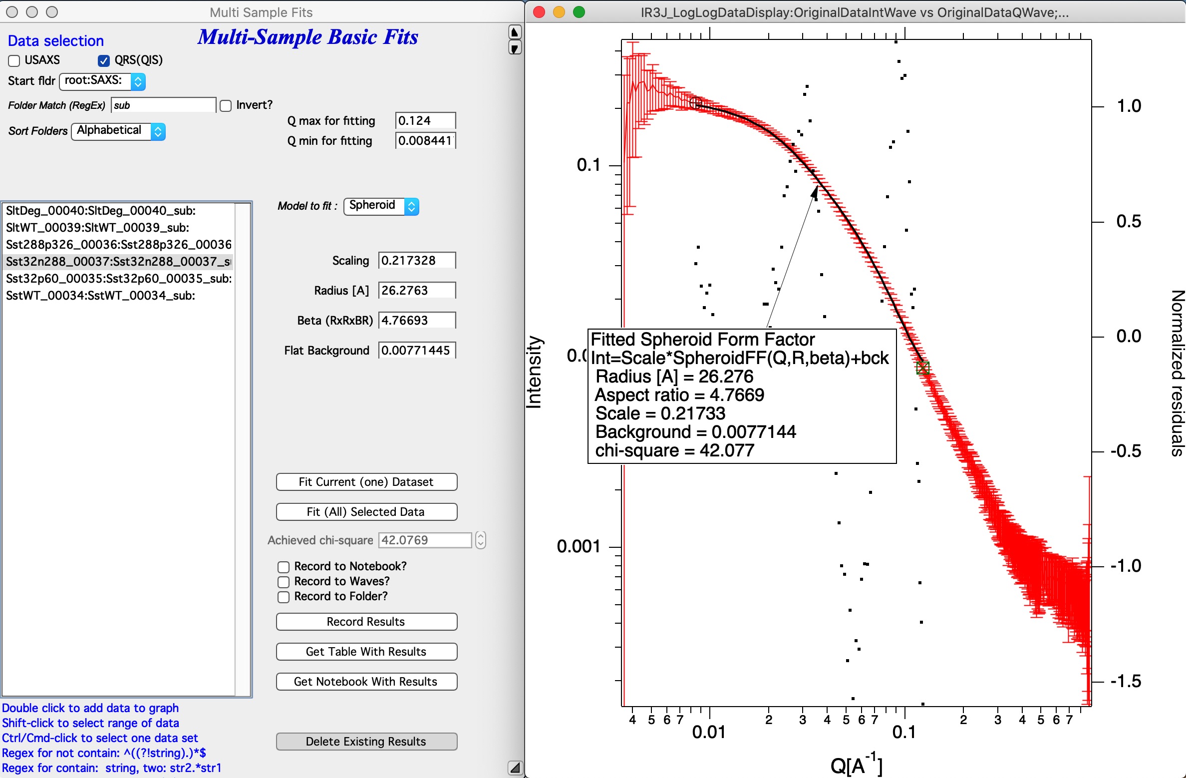
Check the chi-square value as an indicator of goodness of fit.
Saving results
Results can be saved in three ways using the checkboxes on the panel:
Notebook — results are printed to a notebook, opened with the “Get Notebook With Results” button.
Waves — waves containing result values and a text wave with folder names are created in an Igor folder (
root:NameDependingOnMethod). Use “Get Table With results” to display them in a table. These waves can also be plotted manually.Data folder — fitted intensity-Q waves are saved in the source data folder, with fit parameters stored in the wave note. These data can be plotted using Irena plotting tools and the wave notes inspected later using the Metadata Browser.
Run as sequence
Select multiple datasets in the listbox, choose the analysis model, set the Q range, configure result storage, and click “Run on sequence” to process all selected datasets in order (top to bottom as listed). Ordering the data meaningfully (by time, temperature, etc.) produces result tables in a correspondingly useful order.
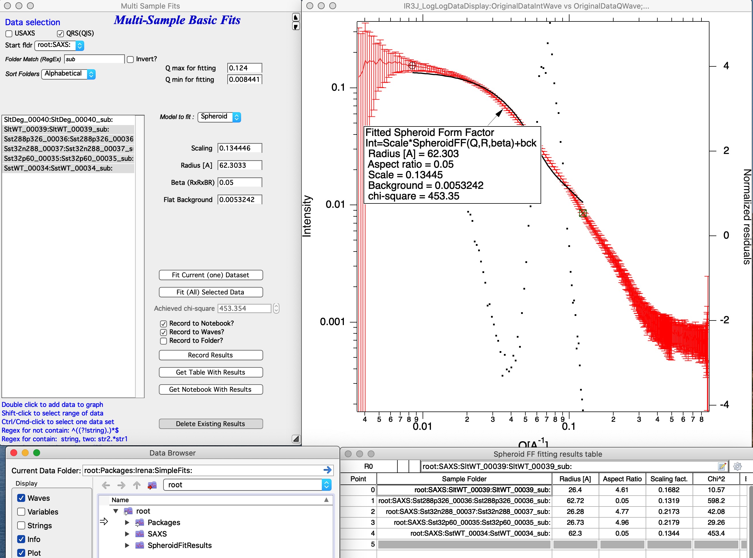
The image above shows results from a Spheroid model run on five datasets.
A new folder root:SpheroidFitResults was created containing waves with
all model results, which were displayed in a table automatically.
“Delete Existing results” — closes the results table and deletes the results folder. There is no undo for this operation.
Models supported
Guinier — Fits the Guinier law.
Porod — Fits Porod’s law.
Sphere — Fits the simple sphere form factor.
Spheroid — Fits the simple spheroid form factor.
Guinier Rod — Fits the Guinier approximation for infinite rods.
Guinier Sheet — Fits the Guinier approximation for infinite sheets.
Invariant — Calculates the scattering invariant with background subtraction.
Power Law — Fits the power law formula:
Invariant
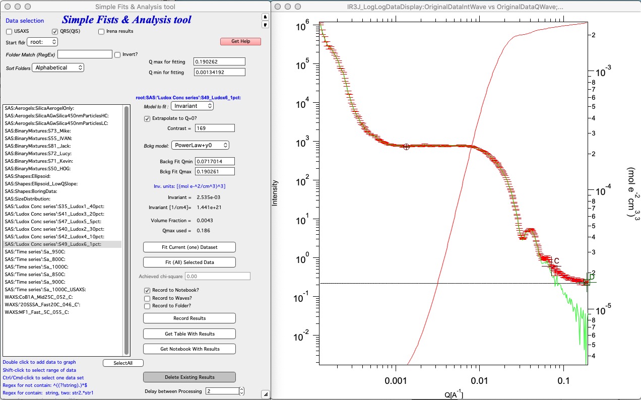
Select “Invariant” and double-click a dataset to add it to the graph. Set cursors A and B (round and rectangle) to define the Q range for the invariant calculation. Enable “Extrapolate to Q=0” when possible. Enter the scattering contrast to obtain results on absolute scale (requires absolutely calibrated intensity data). Select a background subtraction model and use cursors C and D (crosses) to define the range over which the background function is fitted; the fitted background appears as a black horizontal line. Results appear below and can be saved to a notebook or waves.
1D Correlation
Calculates the 1D correlation function, typically used to analyze lamellar structures. Three calculation options are available:
K(z) as reported by Strobl — result in units of (mol e⁻/cm³)². Data scaling may be uncertain in this case; verify carefully.
γ(z) for an anisotropic (highly oriented) lamellar morphology, following Vonk and Kortleve as presented in Roe’s book.
γ(z) for an isotropic lamellar morphology — as in the option above but with a Lorentz-type correction applied to I(q) first (most common case).
Z input (maximum Z in real space) must be in the same units as Q (e.g., nm and 1/nm, or Å and 1/Å). Wavelength input in Å is required; default is the Cu Kα wavelength.
References:
Litvinov et al., Macromolecules 2011, 44, 9254.
Vonk, C. G.; Kortleve, G., Kolloid-Z. Z. Polymere 1967, 220(1), 19–24.
Strobl, G. R., J. Appl. Cryst. 1973, 6(5), 365–370.
Strobl, G. R.; Schneider, M., J. Polym. Sci. Part B 1980, 18(6), 1343–1359.
Roe, R. J., Methods of X-ray and Neutron Scattering in Polymer Science.
Classical electron radius: re = 2.8179 × 10⁻¹⁵ m = 2.8179 × 10⁻¹³ cm.