Reflectivity
This tool models and fits X-ray and neutron reflectivity for up to 8 layers using the recursive Parratt algorithm (L. G. Parratt, Phys. Rev., **95**(2), 359–369, 1954). The underlying code was provided by Andrew Nelson (Andrew_Nelson@users.sourceforge.net). The GUI follows the conventions of the rest of the Irena package.
For more complex fitting than this tool supports, use Andy Nelson’s more capable package Motofit, available at http://motofit.sourceforge.net/ under the GNU license. When publishing results from this tool, cite:
A. Nelson, “Co-refinement of multiple-contrast neutron/X-ray reflectivity data using MOTOFIT,” J. Appl. Cryst. (2006), 39, 273–276.
Optional XOPs for speed
The code supports the optional abeles.xop and GenCurveFit.xop.
Both are optional, but abeles.xop provides a 5–10× speedup. Both can be
downloaded from Andrew Nelson’s website (see above).
Use
A sample 3-column reflectivity dataset is included in the Irena folder
(…Wavemetrics/Igor Pro/User Procedures/Irena/reflectivity.txt). Load it
through the Data loading tool as QRS data.
Select “Reflectivity” from the SAS menu.
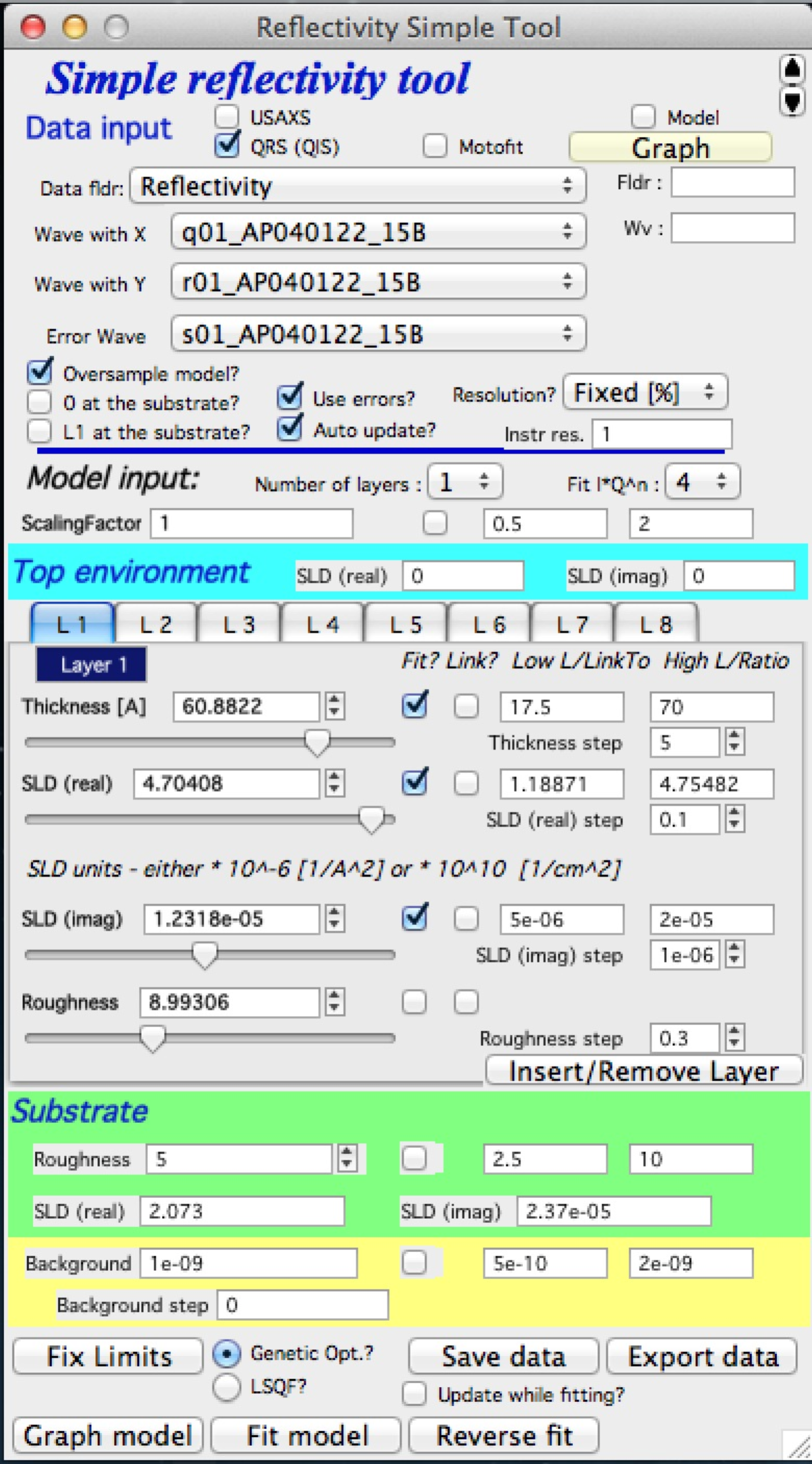
Panel sections:
Standard data selection tools at the top. Select data type, folder, and wave names for Q, reflectivity, and error. Click “Graph” to generate the graphs. For a single-value Q-resolution, uncheck the “Resolution?” checkbox and enter the value; for a Q-resolution wave, select its wave name here. The resolution wave must be in the same folder as the data and must have the same number of points.
Additional options:
“Oversample model?” — calculates the model at 5× the number of input data points. Useful for sparse data (e.g., neutron reflectivity).
“0 at the substrate” — counts thickness starting from the substrate rather than from the top (default is from the top).
“L1 at the substrate” — counts layers from the substrate rather than from the top.
Select the number of layers. Enter the SLD of the top environment (typically air, so 0; for measurements under water, adjust accordingly). Each tab contains controls for one layer: thickness (Å), real and imaginary SLD, and roughness.
Substrate roughness and SLD.
Flat (measurement) background.
Fit control buttons.
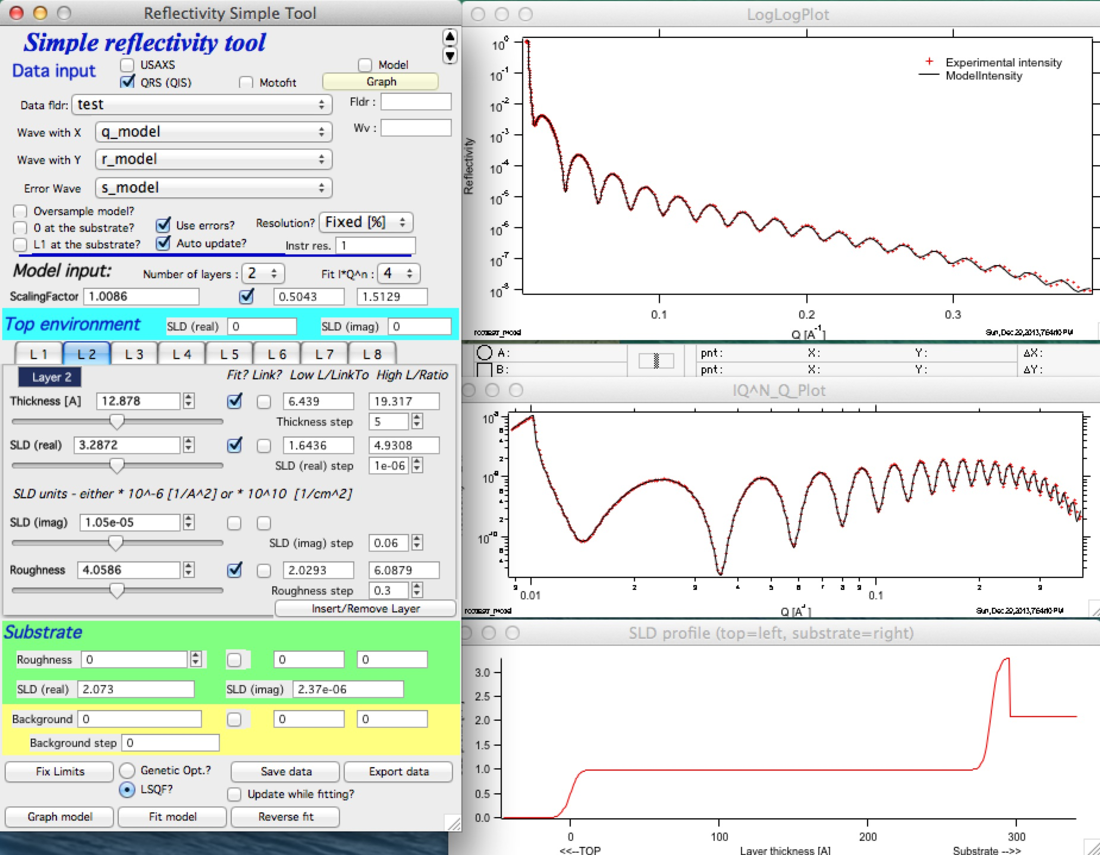
After selecting data, three graphs appear:
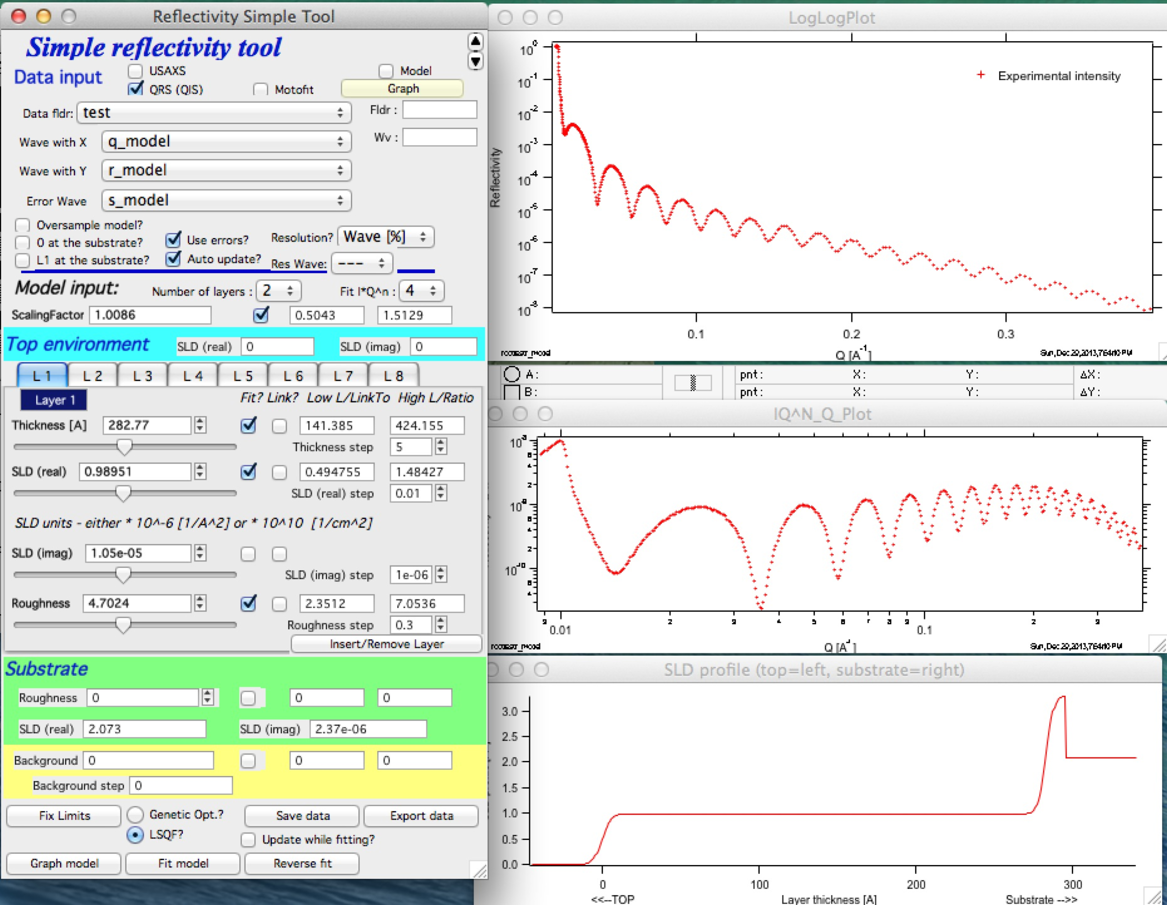
The top graph is a log-log plot of reflectivity vs Q. The middle graph shows reflectivity × Qn (n = 0 to 4, selectable in the panel). The bottom graph shows the SLD profile. Fitting is performed in reflectivity × Qn space to improve numerical stability. Data range selection with cursors must be done in the top (log-log) graph.
Example with known parameters (two-layer system):
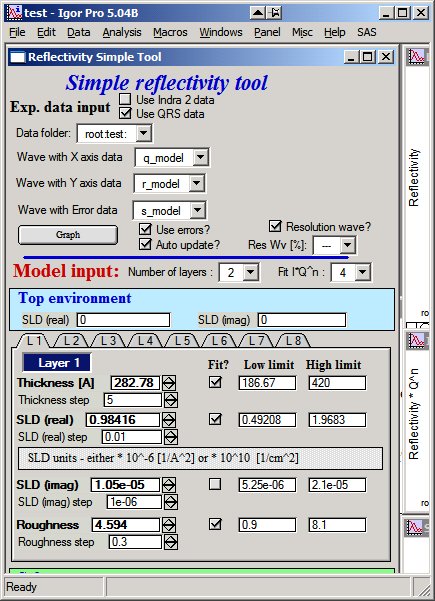
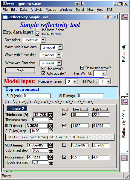
Enter these layer values and a substrate SLD of 2.073 (real part) and 2.37×10⁻⁶ (imaginary part). Set resolution to 1% (uncheck the resolution wave checkbox and enter 1%). Click “Graph model” to compare the model to data:
Adjust parameters to explore sensitivity.
Control details
Resolution wave — Q-resolution input options: fixed percentage (e.g., 1% of Q), a wave containing percentage values per point, a wave containing ΔQ per point, or a wave containing (ΔQ)2 per point.
Auto update — recalculates the model after each parameter change. Required for slider use. Disable on slow computers.
Scale data — apply a scaling factor to match reflectivity to 1 at Q = 0.
Use errors — includes uncertainty values in the fit. Fitting without uncertainties may be unreliable.
Fitting — Select the data range with cursors in the top graph and click “Fit model”. Fitting is performed in reflectivity × Qn space; using n = 4 is recommended to avoid neglecting high-Q data. If the fit fails but reaches a partial solution, “Reverse fit” restores the pre-fit parameters.
For best results, use Genetic optimization. Genetic optimization requires realistic low and high parameter limits.
Insert/remove layer — adds or removes a layer from the current model.
Parameter linking — links two parameters together (e.g., if one is known to be N × another), allowing them to be fit simultaneously.
Save data — copies model data into the data folder for future use. When reloading data from a folder that already contains reflectivity results, the option to restore the previous solution is offered.
Export data — saves an ASCII file for external use. This option is deprecated; the preferred approach is to use “Save data” and then the ASCII data export tool.
Note
For fitting requirements beyond what this tool supports, use Motofit (http://motofit.sourceforge.net/wiki/index.php/Main_Page).