Small-angle diffraction tool
The Small-angle diffraction tool models scattering data using:
Flat background
One Unified level (Guinier + power law)
Up to 6 diffraction peaks
Each peak can have one of many profile shapes: Gaussian, Lorentzian, Pseudo-Voigt, Gumbel, Pearson-VII, modified Gaussian, Lorentz-Squared, or Skewed Normal. Peaks can also represent a Percus-Yevick structure factor S(q) or a Percus-Yevick S(q) multiplied by a sphere form factor F(q).
Use only the peak shapes that are physically meaningful for your system and that you can justify scientifically. Each peak has three parameters: prefactor (scaling, proportional to intensity), position (in Q units), and width (in Q units). Some shapes include a fourth parameter controlling tail height or other shape features. For Pseudo-Voigt, η = 0 gives a pure Gaussian and η = 1 gives a pure Lorentzian.
The tool handles slit-smeared data (USAXS). Two considerations are important for slit-smeared data:
Experimental data should extend significantly beyond the slit length. If the data range ends before the slit length, peaks at Q positions smaller than the slit length must be modeled explicitly.
If ripple artifacts appear (caused by slit-smearing very narrow peaks), enable the “Oversample” checkbox — this increases calculation time by approximately 5×.
Peak position ratios for known structures are collected from:
Block Copolymers: Synthetic Strategies, Physical Properties and Applications, Hadjichristidis, Pispas, Floudas, Wiley & Sons, 2003, chapter 19, p. 347.
Use of the tool
Select “Small-angle diffraction” from the SAS menu.
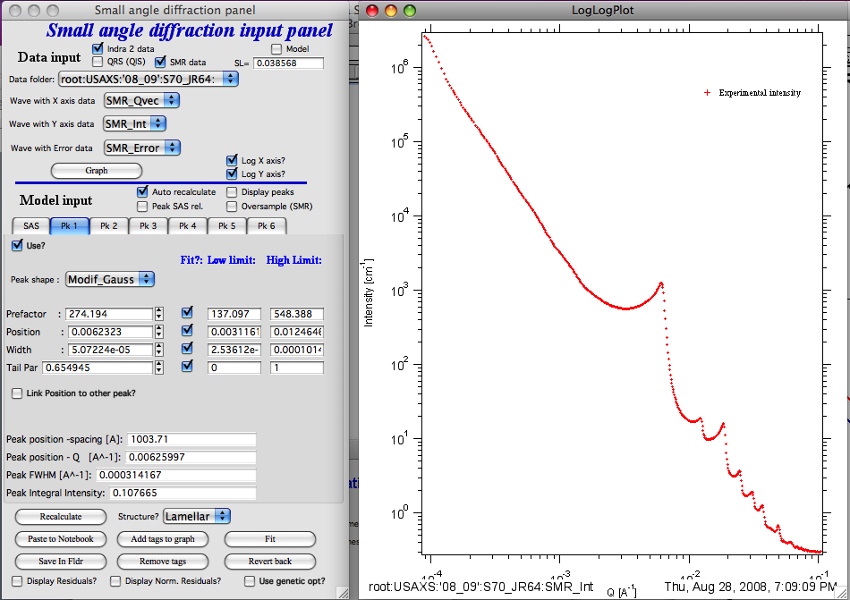
Select data in the data selection controls and click “Graph”. Data are plotted.
Control descriptions
“auto recalculate” — Recalculates automatically after most parameter changes. Uncheck for slow calculations and use the “Recalculate” button manually.
Peak SAS rel. checkbox — This checkbox controls how peak intensities are calculated relative to the Unified fit background:
When unchecked, the model formula is:
When checked, the model formula is:
where Ki is the scaling factor for each peak and F:sub:`i`(Q) is the peak profile Ψ(Q) as a function of the three or four peak parameters.
Interpretation:
Unchecked: assumes peaks and SAS scattering arise from the same population — loosely analogous to an F(Q)·S(Q) assumption.
Checked: assumes peaks are independent of the SAS scattering and arise from different structural features.
The appropriate choice depends on the physical system. Note that fit parameters are always evaluated for Ψ(Q) only — this distinction affects only how the SAS background is applied to the peak amplitude. Diffraction peak profiles are described in Peak Profiles.
“Display peaks” — Displays individual peak contributions. Individual peaks are never slit-smeared.
“Oversample” — For slit-smeared data only. Oversamples the Q range with 5× as many points to reduce artifacts from slit-smearing narrow peaks.
Tab SAS
G — prefactor for the power-law slope
P — power-law slope exponent
Bckg — flat background
Tabs for Peaks
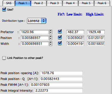
“Use” — enables this peak. Peaks can be used in any order.
“Distribution type” — peak profile shape.
“Prefactor” — peak amplitude scaling factor.
“Position” — peak center position in Q units.
“Width” — peak width in Q units.
“Link Position to other peak?” — links this peak’s position to another peak with a scaling factor (useful for harmonic peaks).
The lower parameter set shows numerically calculated peak properties, which may differ slightly from the direct input parameters.
Final controls
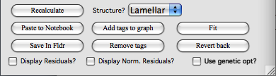
“Use genetic optimization?” — uses genetic optimization. Very slow; unlikely to be needed for this tool. See explanation in the relevant chapter.
“Fit” — runs the least-squares fit.
“Revert back” — restores parameters to their pre-fit values.
“Add tags to graph” — adds parameter annotations to the graph.
“Remove tags” — removes annotations from the graph.
“Structure?” — sets peak position ratios for known mesophase structures. Peak 1 position is the reference; remaining positions are set as fixed multiples. Widths and prefactors must be set manually.
“Save in Fldr.” — saves results (and peak profiles if selected) to the data folder.
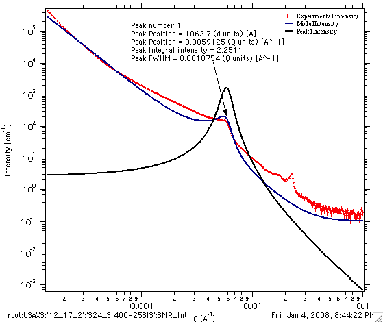
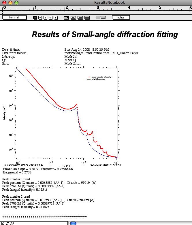
“Paste to Notebook” — opens the results notebook and pastes the graph and a results summary.
“Recalculate” — forces model recalculation.
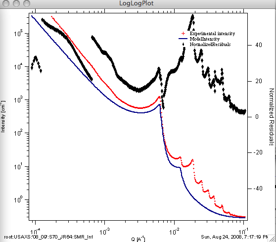
Residuals or normalized residuals can be appended to the graph:
Note
Verify that fitting parameter ranges are set appropriately before running a fit — incorrect limits are a common source of poor fits. All fit results are also automatically recorded in the Irena SAS logbook.