Mass Fractal Aggregate model
This tool generates a 3D random representation (voxelgram) of a mass fractal aggregate. For details on the underlying science, see:
A. Mulderig et al., “Quantification of Branching in fumed silica,” J. Aerosol Science 109 (2017) 28–37. http://dx.doi.org/10.1016/j.jaerosci.2017.04.001
This tool is applicable only to mass fractals. Understanding the limitations and the meaning and reliability of the fractal parameters is essential before use.
Warning
This is a visualization tool, not a fitting tool. Data must first be fitted with Unified Fit. Assuming a mass fractal structure, fractal parameters describing the system are extracted. The tool then uses Monte Carlo methods to randomly generate one of many possible shapes consistent with those parameters. Running the tool with the same parameters will produce a different shape each time.
Keep in mind:
Results are stochastic. Store acceptable results — they may be difficult to reproduce exactly.
Occasionally the code produces errors or hangs during evaluation of an aggregate. The solution is to run the model again. Some specific parameter combinations may consistently fail; try different parameters.
“Find Best Match Aggregate” (added 2021/12) — runs repeated random growth of aggregates and evaluates each against a target Misfit parameter (see definition below). Growth stops when an aggregate within the target Misfit is found or when the maximum number of attempts is reached.
Mass fractal model parameters
Following: http://dx.doi.org/10.1016/j.jaerosci.2017.04.001
A mass fractal aggregate is described by:
R — aggregate size
df — mass fractal dimension
p — short circuit path length
s — connective path length
dmin — minimum path dimension
c — connectivity dimension
These parameters are inter-related by:
Where:
Rg is the radius of gyration of the second (large) Unified Fit level — represents the mass fractal aggregate size.
dp is the Sauter mean diameter of a sphere with similar surface-to- volume ratio as the primary particle (first, smaller level).
The value z (degree of aggregation), dmin, and c are calculated by the Unified Fit “Analyze results” function. df is the power-law slope of the second (larger) Unified Fit level for a mass fractal represented by two levels.
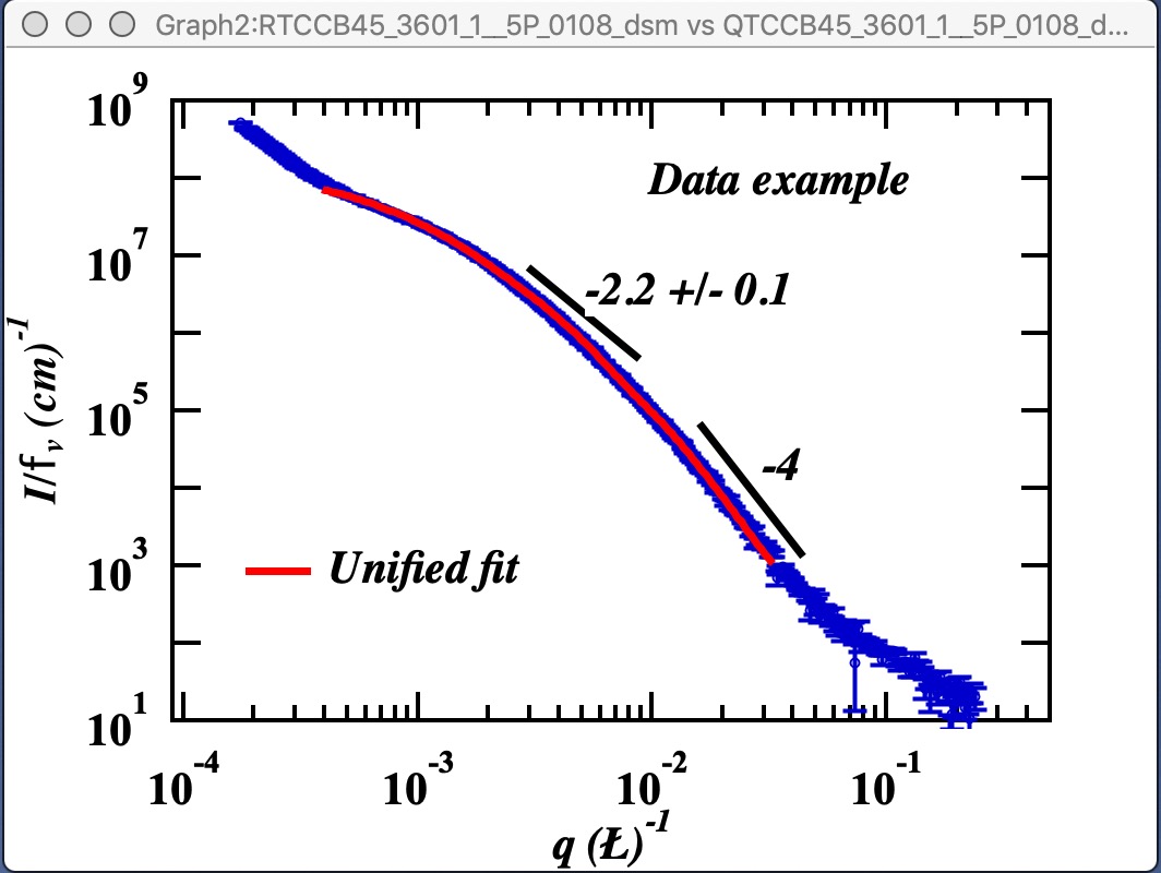
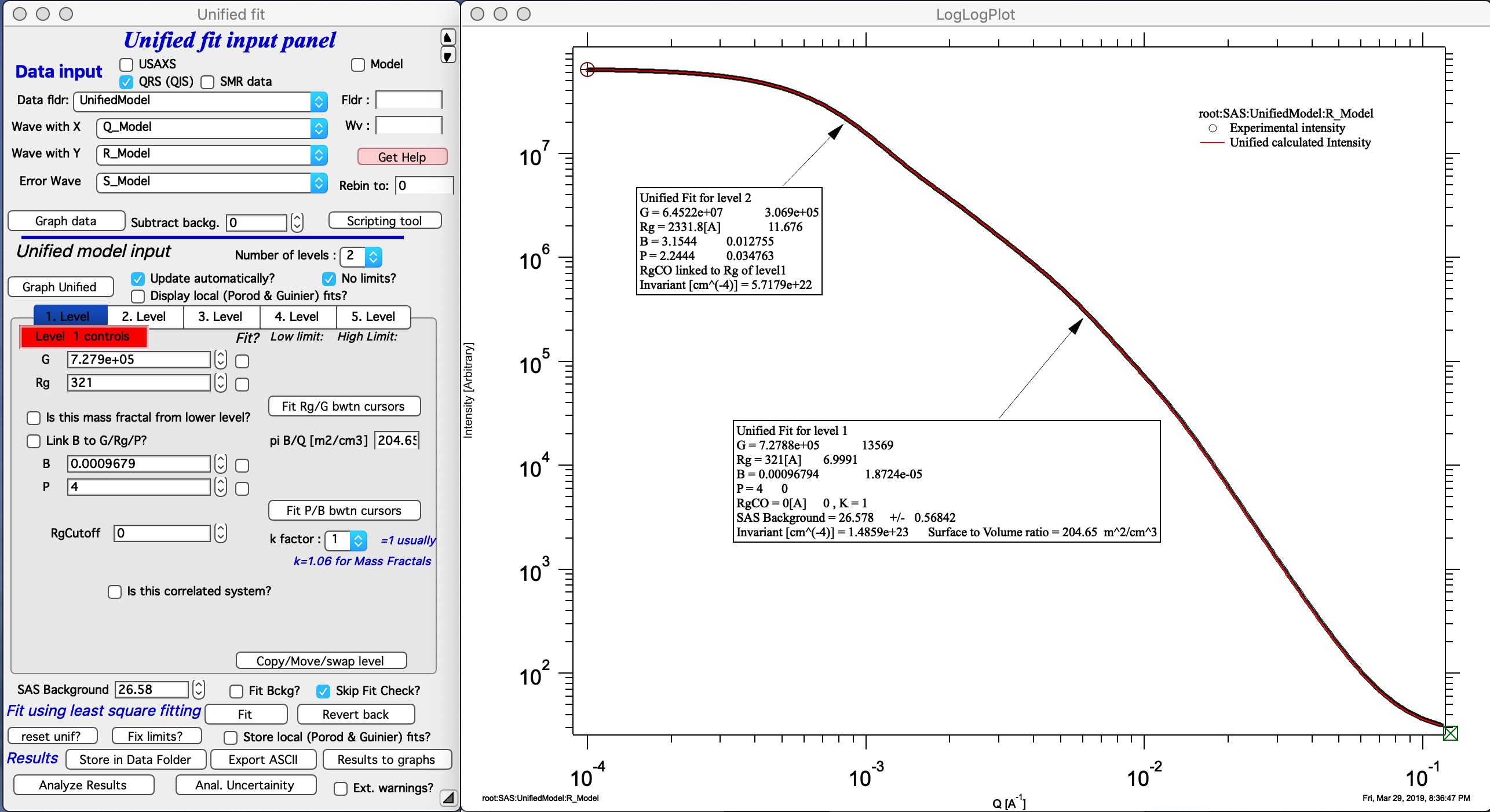
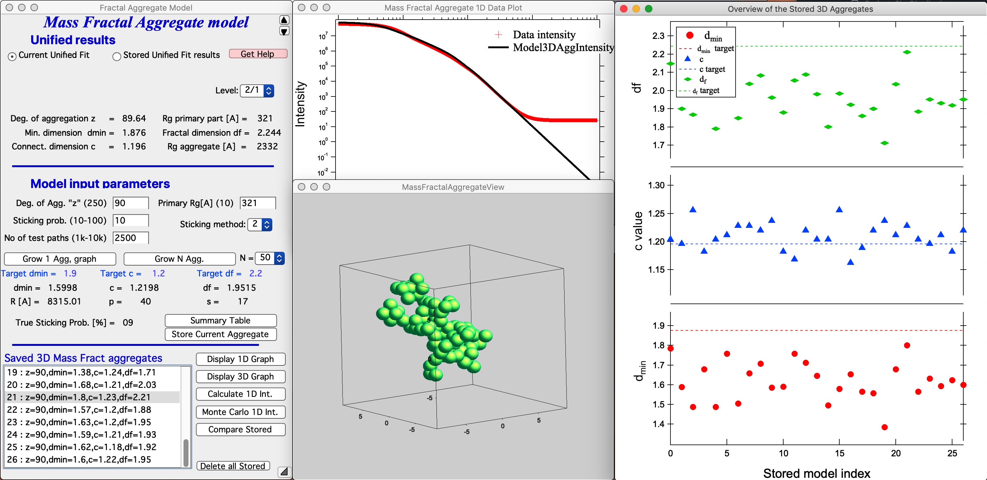
Example: data with an associated two-level Unified Fit (primary particle Rg ≈ 320 Å, mass fractal dimension ≈ 2.23, aggregate Rg ≈ 2332 Å):
With Unified Fit results available (either from the current fitting state or stored in the data folder), open the Mass Fractal Aggregate tool:
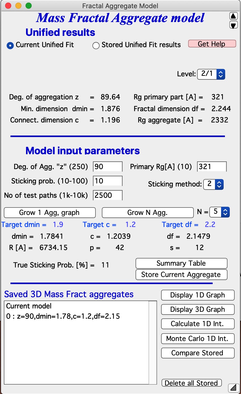
The top section offers options to use results from Unified Fit. Data can be selected from stored results or from the current Unified Fit working directory. By default, levels 2/1 represent the mass fractal; change via the “Level” popup if needed. Values update when the Level popup is changed. The extracted parameters are shown in a table; the most important values (target z and df) are repeated in blue below “Grow Aggregate”.
Growth control parameters
Degree of aggregation (z) — number of primary particles in the aggregate.
Sticking probability (SP) — probability that an arriving particle sticks to the aggregate (10–100%).
Sticking method (1, 2, or 3) — defines the minimum distance for sticking in the cubic lattice:
1 — nearest neighbor in one axis direction (distance 1)
2 — includes in-plane neighbors (distance √2)
3 — includes body-diagonal neighbors (distance √3)
Multi Particle Attraction — controls how the presence of multiple neighbors modifies the sticking probability:
Neutral — probability independent of neighbor count.
Positive (Attractive) — more neighbors increase probability. (SP for 1 neighbor = user value; for 2 = (SP+100)/2; for ≥3 = (SP+300)/4)
Negative (Repulsive) — more neighbors decrease probability. (SP for 1 = user value; for 2 = (SP+10)/2; for ≥3 = (SP+30)/4)
Not Allowed — more than one neighbor prevents attachment. (SP for 1 = user value; for 2 = 1%; for ≥3 = 0%)
Repulsive/Not Allowed settings produce larger, more open aggregates; Attractive settings produce more compact aggregates.
General guidance:
Compact aggregates (high df, up to ~2.55): sticking method 1, low SP, Attractive.
Open aggregates (low df, below ~1.8): sticking method 3, high SP, Repulsive or Not Allowed.
Note: larger z values significantly increase computation time. Monitor the history area for progress and final parameters.
“Max paths/end” — maximum number of path-tracing attempts from each endpoint used to compute the fractal parameters. Higher values give better statistical accuracy but take longer. A value of ~1.5k is a reasonable default; for larger aggregates (high z), this limit may be reached before all paths are found.
“Primary Rg [Å]” — primary particle radius of gyration. Sets the real-world scale of the aggregate.
Growing aggregates
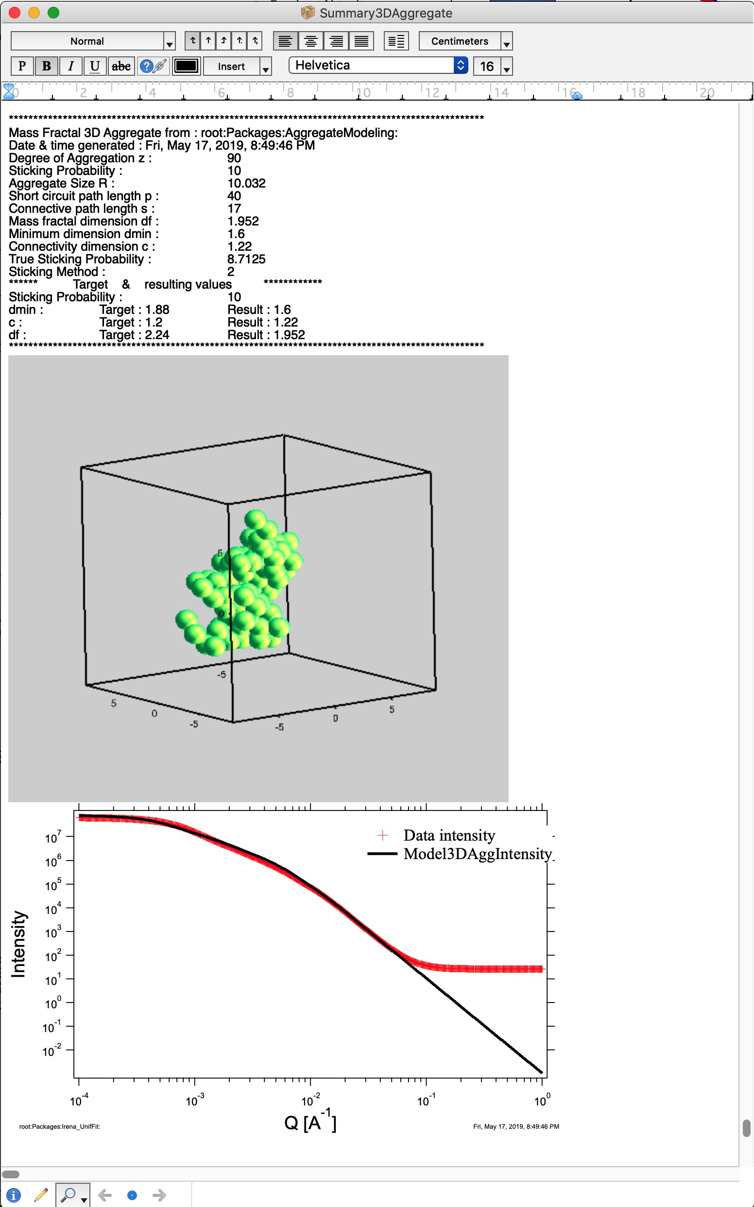
Click “Grow 1 Agg, graph” to generate and display one aggregate in Gizmo and compute its 1D intensity for comparison with the source data. Computation takes a few seconds for typical parameter values:
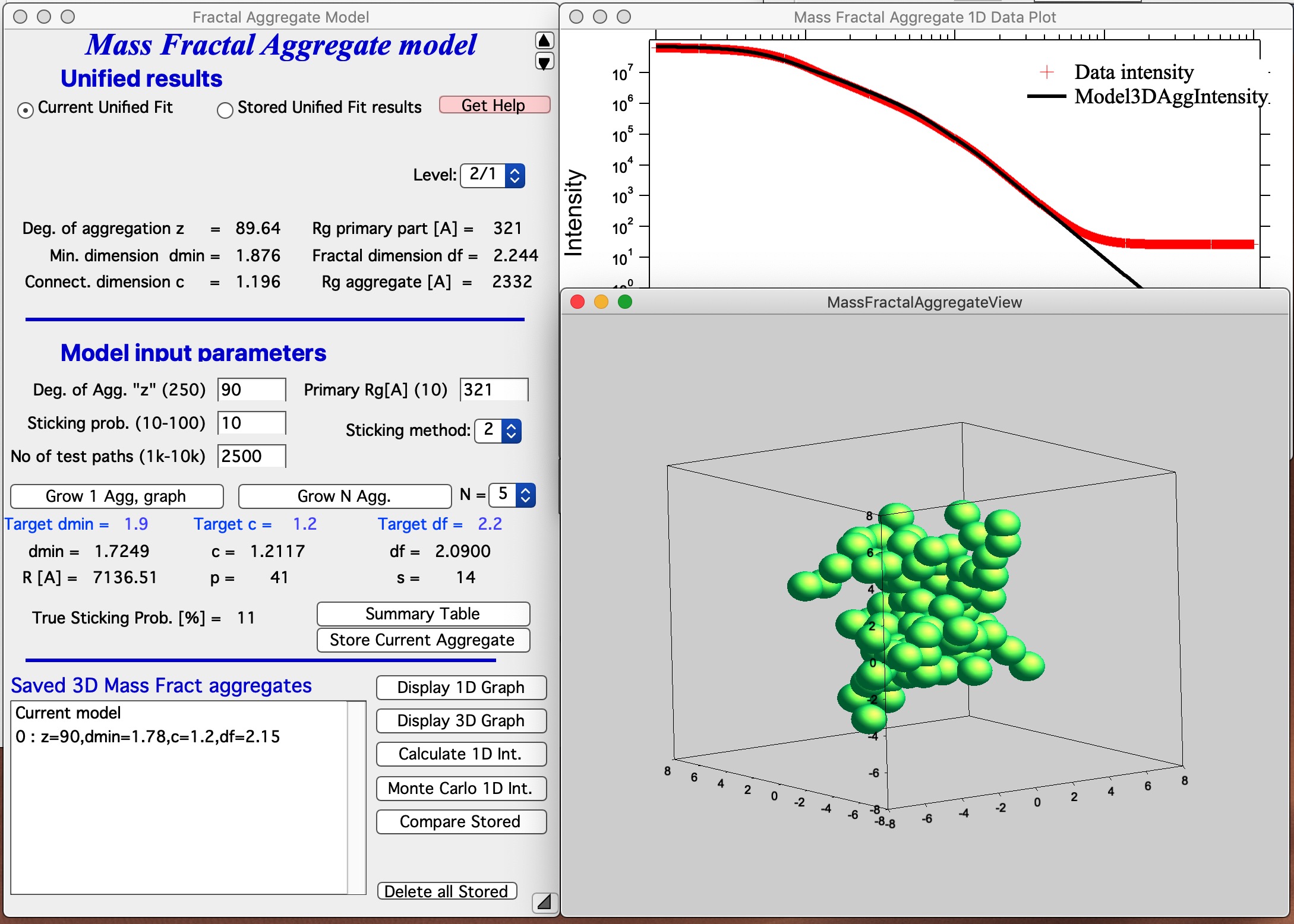
A result within parameter uncertainties is generally acceptable. Parameters will rarely match exactly — for example, if df from Unified Fit has an uncertainty of ±0.1, matching to that precision is not meaningful.
Click “Grow N Agg” to generate N aggregates sequentially (default N=5, max N=50). Each result is displayed in Gizmo, the 1D intensity is calculated and overlaid, and the summary is saved to a notebook. Aggregates that fail during growth (too compact) are skipped; the final count may be fewer than N.
“Summary Table” — displays a notebook with model summaries and appends the current result. Use this to track how parameters depend on growth settings.
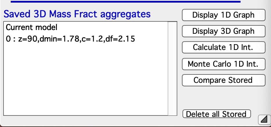
“Store Current Aggregate” — saves the current aggregate (including 3D data) to a separate folder and adds it to the Saved 3D Mass Fract Aggregate listbox:
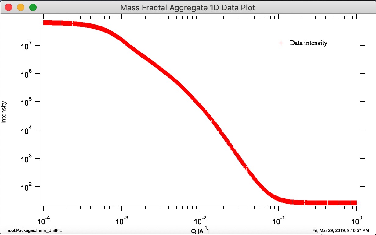
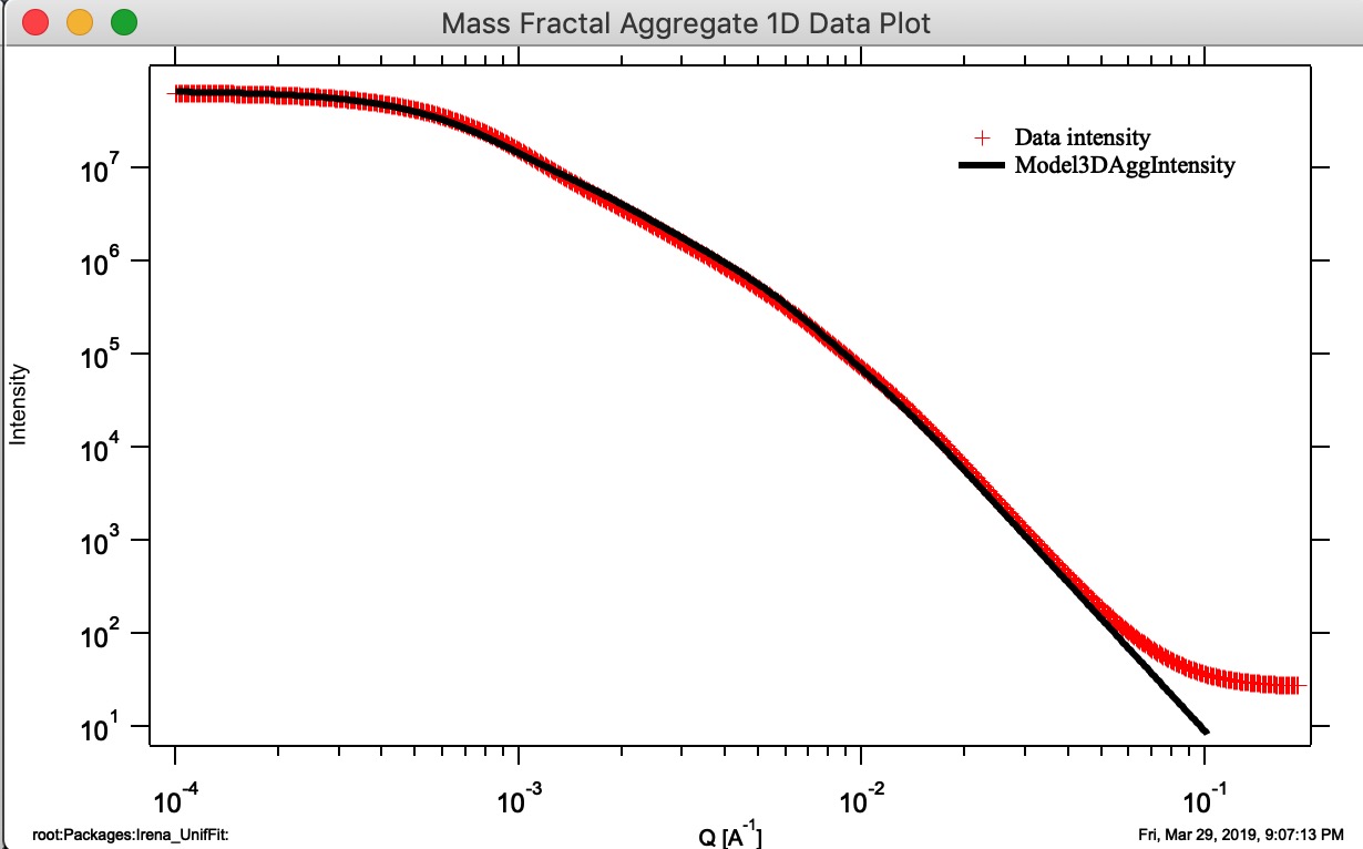
“Display 1D graph” — loads Q/Intensity data from the source folder and creates a “Mass Fractal Aggregate 1D Data Plot” graph:
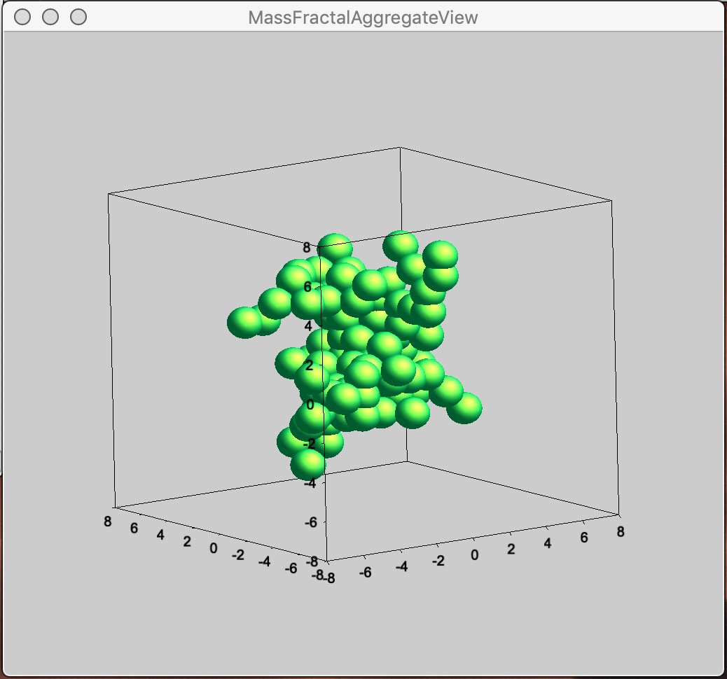
“Display 3D graph” — displays the selected result in Gizmo:
“Calculate 1D Int.” — calculates the 1D intensity from aggregate parameters and appends it to the 1D graph. Intensity is normalized to match the measured data over the middle Q range. This model predicts the shape of the 1D curve, not absolute intensity:
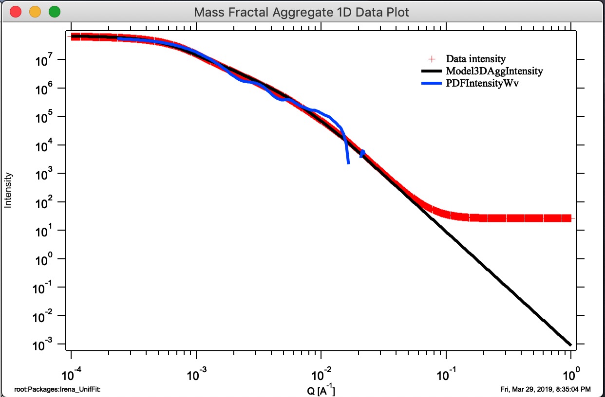
“Monte Carlo 1D Int.” — computes 1D intensity by Monte Carlo sampling of the pair distance distribution and appends the result to the 1D graph.
Note
The Monte Carlo 1D intensity calculation is slow, noisy at high Q, and not very representative. It is useful mainly as a consistency check but is not recommended for routine use.
“Compare Stored.” — plots df, dmin, and c for all stored aggregates, enabling selection of the result closest to the target:

In this example, model 21 best matches the target df and dmin values. Selecting it in the listbox and generating 3D and 1D graphs:
“Delete all Stored” — deletes all stored 3D aggregates and closes associated graphs.
Find Best Match Aggregate
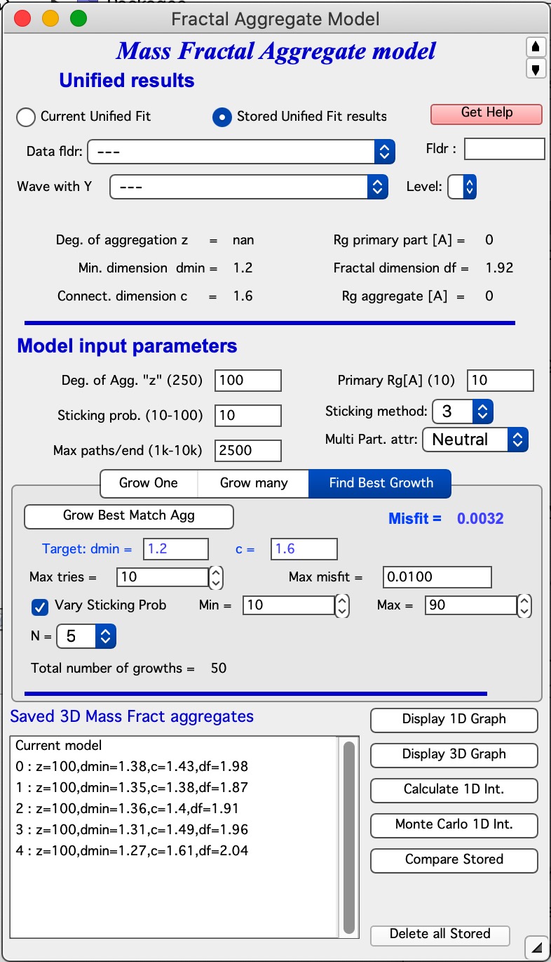
This function automates the search for an aggregate that matches the target fractal parameters within a specified Misfit tolerance.
How to use:
Set the blue target fields “Target d:sub:`min`” and “c” (loaded automatically from Unified Fit, or entered manually).
Set the target “Misfit” value. A value of 0.01 is a good starting point.
Set the maximum number of aggregates to attempt per sticking probability (default: 10).
Choose whether to vary sticking probabilities across a range (default: no; if yes, 5 steps between 10% and 90%).
Set sticking method and multi-particle attraction.
Click “Grow Best Match Agg”.
The code grows aggregates until either the maximum total count is reached (default 50) or an aggregate within the target Misfit is found. The best result (lowest Misfit) is available at the end.
Misfit values are included in the Compare Stored output and notebook records.