Bio SAXS support
List of Tools
Import bioSAXS ASCII Data
This chapter describes how to import bio SAXS 1D SAS in Irena. Irena has other importers - for ASCII, HDF5 canSAS Nexus, & canSAS XML - suitable for most non-bio type data. These are described here Import Data
Users of Indra 2 or Nika produced data can skip this chapter.
Function description:
This ASCII 1D data loader is custom made for specific ASCII data type. Please check that your data are compatible with these requirements.
ASCII with two or three columns of data. Optional text block separated by separator (many different supported) will be skipped and ignored.
First column Q vector in [1/Angstrom], optionally in [1/nm] which can be converted into [1/Angstrom] which Irena uses.
Second column Intensity (ideally absolute, but relative is fine)
Third column (optional) is uncertainty (error) for intensity. If there is no uncertainty, it will be created as 4% of intensity value.
Typically (optional) more files per one sample, files are designated by “_00001” number at the end of the name (number length does not matter, separator _ is required). All characters before this last number are considered sample name.
Sample names are unique and not excessively long. Suggested limit is 20-25 characters or less. This is GUI limit, not Igor 8 limit.
Default extension expected is dat, but can be changed in the GUI.
Example of valid names
Buffer_01 measurements:
    Buffer_01_00001.dat, Buffer_01_00002.dat, Buffer_01_00003.dat, etc...
Sample1_035 measurements:
    Sample1_035_000001.dat, Sample1_035_000002.dat, Sample1_035_000003.dat, etc.
Example of valid data file content
% Filename : Sbuf1_00033_00003.tif
% Date & Time : 19-Feb-2020 15:24:09
% X-ray Energy (keV) : 13.300
% Exposure Time (s) : 0.500
% Beam Center : 741.50700, 216.72300
% Sample to Detector Distance (SDD) (mm) : 2007.410
% Detector Pixel Size (mm) : 0.172
% Photodiode Value : 15670.500
% I0 of Sample : 1.244850e+04
% I0 of Standard : 1
%
% q(A^-1)   I(q)    sqrt(I(q))
3.50000000e-03 0.00000000e+00  0.00000000e+00
3.62054899e-03 1.76072986e+00  1.28270598e+00
3.74524999e-03 1.27342930e+00  6.58838643e-01
3.87424601e-03 1.59209666e+00  1.10772011e+00
etc.
Importing ASCII SAS data
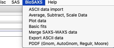
Select ASCII data import from “BioSAS” menu. You get GUI, which presents various options described below.
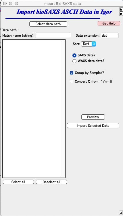
Explanation of control available here:
“Select data path” browse to the folder on the computer drive where the data for import are located.
“Data path” this shows the path selected above. Cannot be edited in this window, use button Select data path to change the path if needed.
“Match name” enables to use string to show in the listbox only subset of files.
“List of available files” lists all files in the current folder on the computer, unless masked by Data extension. One or more files here can be selected for import. Use shift - click to select multiple files (on Windows) or cmd – click on Macs (to pick one file at time), shift-click to pick range of files. Double click on file runs “Test” and “Preview” commands on that file.
“Data extension” if extension is put in this filed (e.g., “dat”) only files with the “dat” extension will be shown in the List of available files.
“Preview” Test import of first selected file. Not really necessary, but very useful. Will display graph, if it looks OK, you should have no problems reading the files.
”Select all” or “Deselect all” modifies which files are selected in “List of available files”.
”SAXS data?” or WAXS data? select if you are importing SAXS or WAXS data. All this does is it places data folders in either root:SAXS or root:WAXS folders for easy orientation. It also enables you to have same file names for SAXS and WAXS data. NOTE: You can merge SAXS and WAXS using Irena Merge data tool.
“Convert Q from [1/nm]” select if units used in file for Q are [1/nm]. Units will be converted to A-1 if nm-1 data are imported. Irena uses A-1.
“Note on errors” if the data imported do not contain error bars, this tool will generate 4% Intensity errors.
NOTE: If the data contain header of data (typically number of lines with special character, such as #, $, … at the start of the line and some spaces before useful information, this ASCII importer will simply ignore them.
Use of the ASCII Import tool:
Locate data using “Select data path” button. This will populate the listbox on the left hand side. Double click any file to generate preview graph (or select file and push button “Preview” which will do the same thing). If the graph looks OK - check the Q units at this moment - the tool will import the data without issues. If there are weird things and something does not look right, you can try using Irena ASCII importer in menu SAS>Data Import Export>Import ASCII SAS Data. It has lot more functionality and you can probably import the data that way. read the manual on this tool…
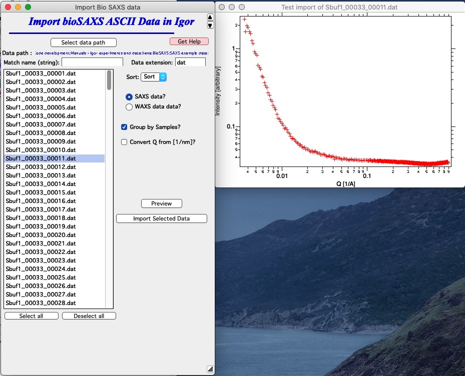
So, lets assume the graph looks OK. Check the Q scale - in case the Q values are 10x larger than you expect, you have Q in 1/nm and need to check the checkbox “Convert Q from [1/nm]” Select files which you want to import - or just select all using button “Select all”.
Next decide, if you have many files per one sample - typically multiple measurements you want to average first - or if you have one file per sample. If you have many files (our example) you should check “Group by Samples?” option. If you have one file per sample, you should uncheck this checkbox or your data structure will be too complicated.
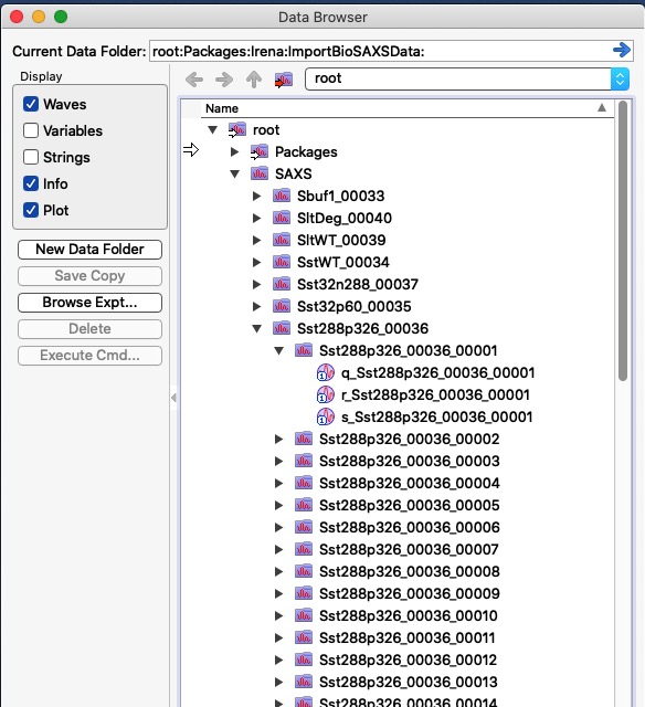
If the “Group by Sample?” is checked, code will assume that string before the last number separated by “_” - that is before “_00023.dat” is the name and create subfolder for that sample. That is VERY convenient in this case, you’ll see it later. See in the image below, how the data structure looks like: your data were imported in root:SAXS. In there, for each sample name code created folder with name based on the file name (without the last “_000xx” number). It placed all individual data inside its own folders with names which now2 include that last number to make sure the names match the file names. Inside each individual folder code placed your q values in wave called “q_sampleName”, intensity in “r_samplename” and errors in “s_samplename”. This is what is knowns as QRS naming system Irena uses QRS naming system.
However, if you have only one measurement per sample, using this grouping just buries your data to deeper folder structure. In that case, do NOT do it, it will just keep annoying you.
BioSAXS Data manipulation - Average, Subtract, Scale
This chapter describes how to use Average, Subtract, Scale tool for bioSAXS data. Irena has other Data manipulation tools. These are described here Data Manipulation 1 and Data Manipulation 2
This tool is used to :
Average multiple measurements on single sample to get averaged data set. This is used to obtain better statistics. If you have just one measurement on a sample, skip Average step.
Subtract buffer measurement from sample measurement. Buffer can be scaled if needed for transmission.
Scale data if needed. This simply scales intensity and Error (uncertainty) by value provided by user. For example, if data need to be placed on absolute intensity scales and calibration constant has not been yet applied.
Using default naming of data sets here is important Naming folders with data is critically important to keep user sanity. You can get easily in situation, that you have no clue what data are where and result is mess and errors. Try to use default names and you have chance to keep your sanity.
Naming of files
After import, you should have one or more data files imported. If you have multiple measurements for each sample, your data should be in:
root:SAXS:SampleName
and inside this folder should be multiple folders named similarly to: SampleName_0001, SampleName_00012, SampleName_0003, SampleName_0004, … These are multiple measurements which now need to be averaged.
After Averaging, the code will create a new folder with data called SampleName_ave inside the root:SAXS:SampleName folder.
After Subtracting buffer the code will create a new folder with data called SampleName_sub inside the root:SAXS:SampleName folder.
After Scaling data the code will create a new folder with data called SampleName_sub_scaled inside the root:SAXS:SampleName folder.
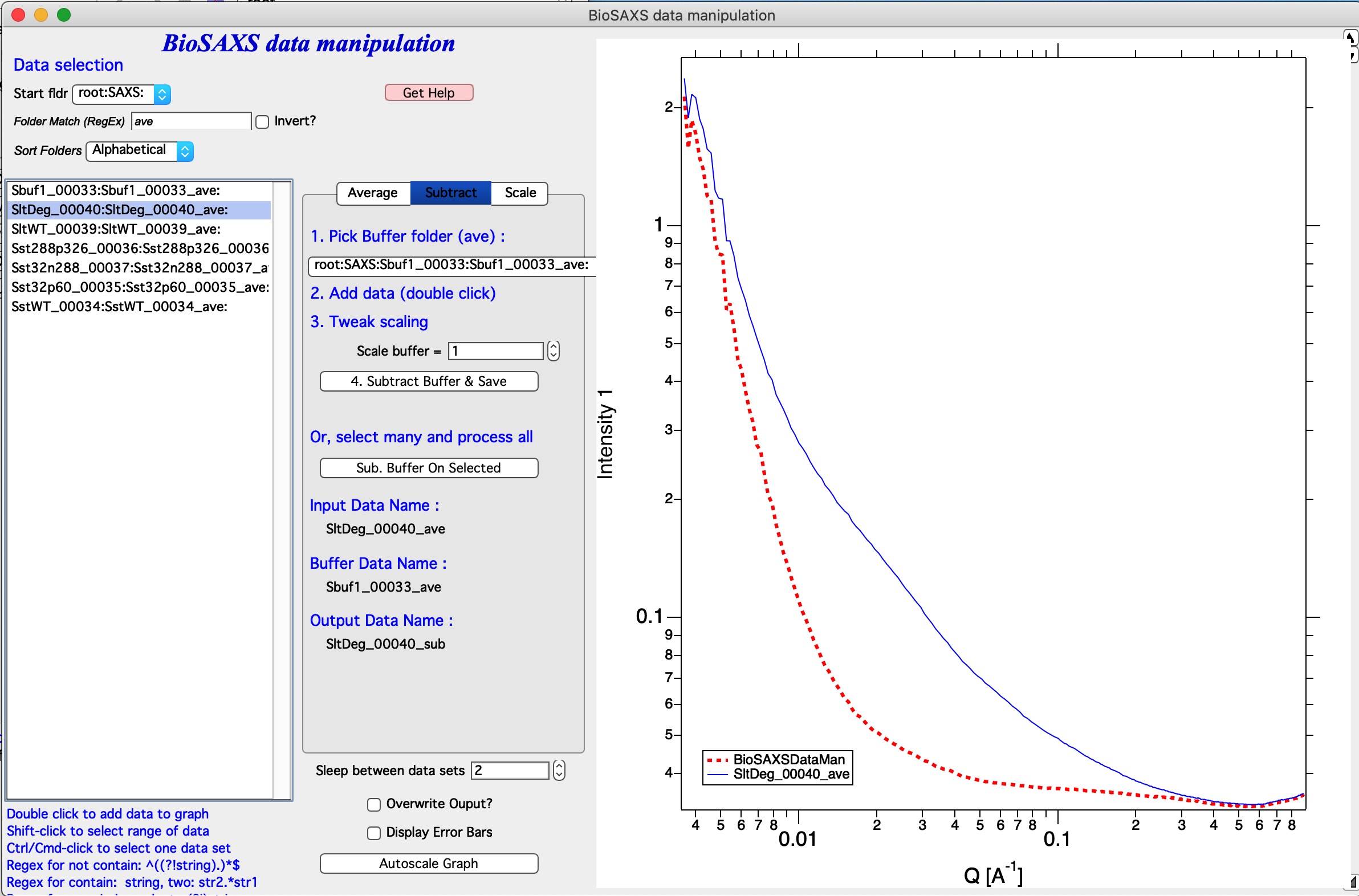
The main GUI is here:
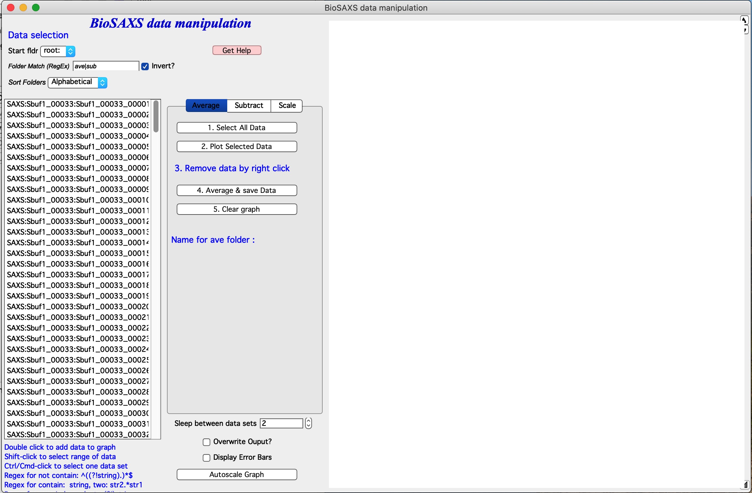
The tool can do three things quickly and easily… It is not meant for more complicated processing. It also assumes, that you follow the procedure in order - Average - Subtract - and optionally Scale. Any other order may cause major troubles.
Selecting data
Understanding data selection tools makes user life easier. In the Data selection part of the panel you need to define sufficiently the data you want to look inside. There is detailed description on how to use this widget system Multi Data selection. Please refer to that page for details.
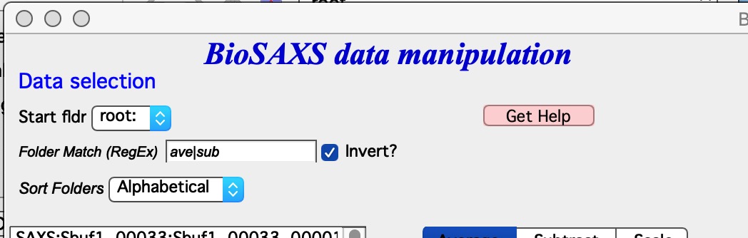
Start Fldr. Here you can select at which location in data tree code will start looking for the data. In this case the code looks for data from root: Folder Match (RegEx) this allows us to look for only some of the folders. A short summary on regular expressions is at the bottom of the page, below the Listbox with folder. Google it, understanding regular expressions will be very helpful. Invert? this checkbox inverts the Regular expression meaning. Sort Folders This sorts the folders using one of many methods implemented. As result, this will group folders in order which may be helpful for processing.
HOW TO USE Pick a good starting folder. If you select root:SAXS: folder, it will show you all data inside this one folder - inside all subfolders. For example, selecting root:SAXS: exposes 7 folders × 45 measurements each — a large list. Selecting instead root:SAXS:Sbuf1_00033: as the starting folder shows only the 45 relevant datasets.
Also, note that code automatically puts “ave|sub” and checks the “Invert?” checkbox. This will prevent, if they would happen to exist, folders generated by this averaging and by subsequent subtracting of buffer from showing up and being accidentally averaged. This is useful when you are reprocessing the data.
Average
The purpose is to add all measurements in the graph, evaluate if all measured data should be averaged, remove any which for whatever reason should not be included and then average those which user approves.
Adding data
To add data, there are two options.
Add by double click if you double (left) click on a name of data set, it will be added to the graph. Note: each data set can be in the graph only once and subsequent attempt to add it again will simply be skipped.
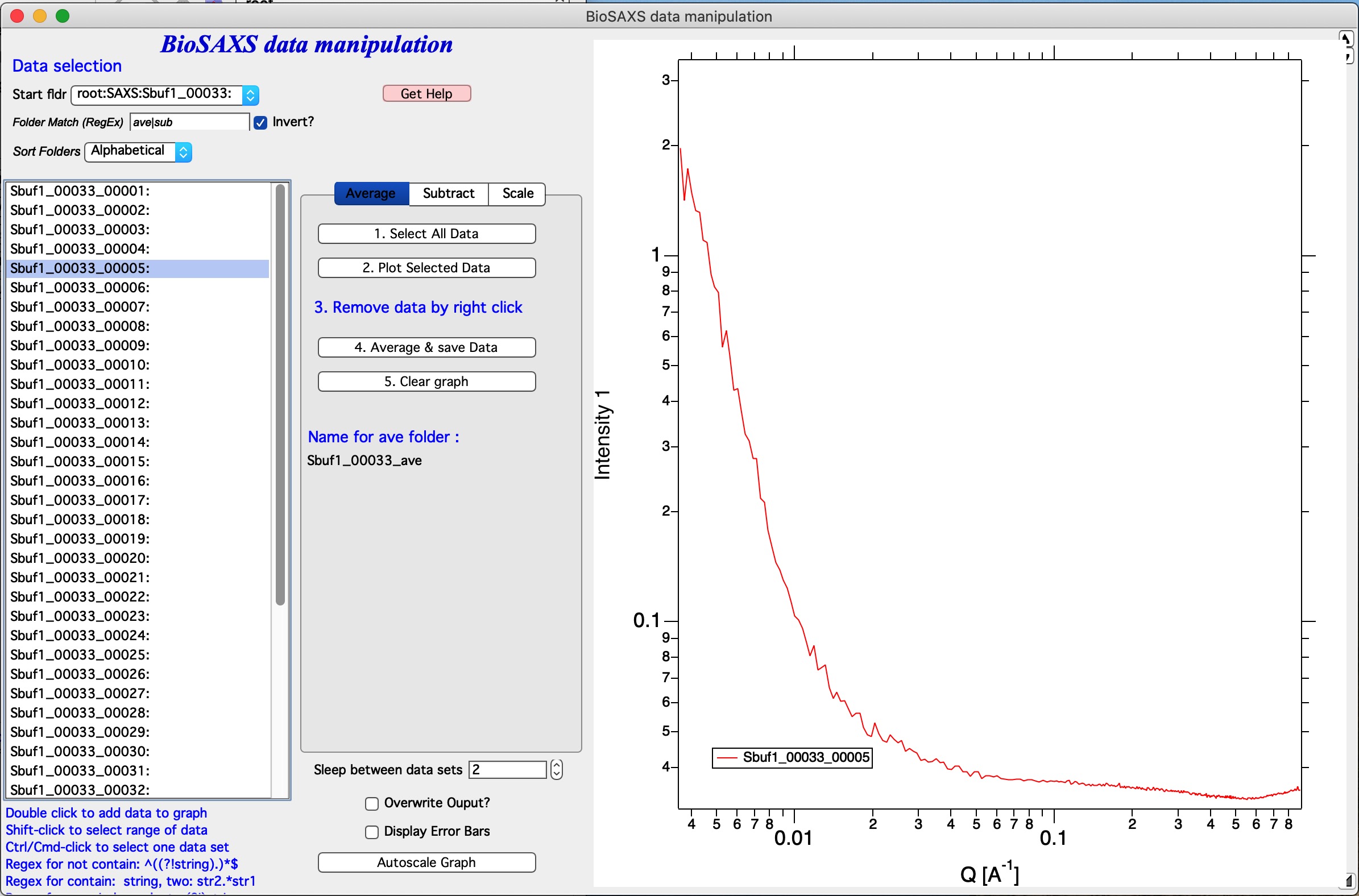
Double-clicking on Sbuf1_00033_00005 adds it to the graph. You can add as many datasets as needed, though adding many individually becomes tedious.
Add as group This is more likely expected use. In the listbox now we have ONLY measurements related to one sample. This is because the start folder is set to root:SAXS:Sbuf1_00033: and two other types of data sets there (ave and sub) are hidden using the Folder Match controls. We can therefore follow the buttons and their order to get more productive. Here is correct easy to follow procedure:
Select the Start folder to point to one sample set of measurements.
Hit button 1. Select All Data, this will select all data in the listbox. You can deselect the data you know you do not want now - hold down control/command key and click on names you do not want.
Hit button 2. Plot Selected Data. This will add all selected data into the graph and create legend.
Now you can decide if any are outliers which need to be removed. Remove the data sets by right click and “Remove XYZ_wave_name”. If needed, zoom in using Igor graph tools (left click-drag create Marquee and right click inside, select Expand). To autoscale back use Autoscale Graph button at the bottom of the panel. Once you removed all data sets which you do not want to include, continue…
Hit 4. Average & save Data button. This will average all data together and create a new data set with SampleName_ave name inside the SampleName folder.
(Optional) Hit 5. Clear graph this will remove all data from the graph. It is optional if next you would use buttons from the start of this procedure, button 2. Plot Selected data does remove the old data first anyway.
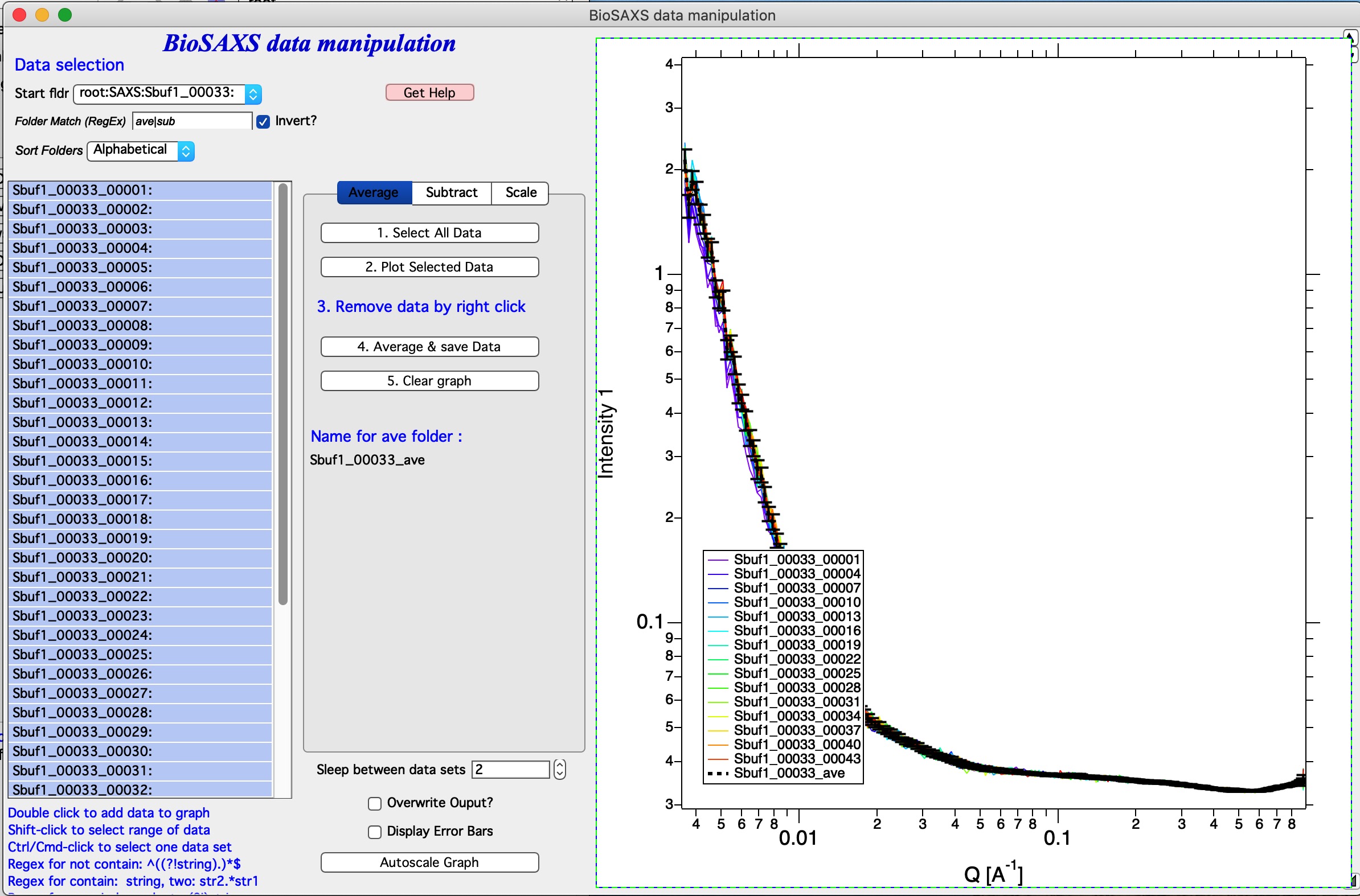
In the graph code adds the black averaged data set and saves the data.
Now, to process all of the imported data all I have to do is to follow the above routine for each imported set of 45 measurements per sample. Note, that the code is writing report in the history area of Igor (just above command line input):
Created averaged data set in:root:SAXS:SltWT_00039:SltWT_00039_ave: Averaged following data :
sets:r_SltWT_00039_00001;r_SltWT_00039_00002;r_SltWT_00039_00003;r_SltWT_00039_00004;r_SltWT_00039_00005;r_SltWT_00039_00006;r_SltWT_00039_00007;r_SltWT_00039_00008;r_SltWT_00039_00009;r_SltWT_00039_00010;r_SltWT_00039_00011;r_SltWT_00039_00012;r_SltWT_00039_00013;r_SltWT_00039_00014;r_SltWT_00039_00015;r_SltWT_00039_00016;r_SltWT_00039_00017;r_SltWT_00039_00018;r_SltWT_00039_00019;r_SltWT_00039_00020;r_SltWT_00039_00021;r_SltWT_00039_00022;r_SltWT_00039_00023;r_SltWT_00039_00024;r_SltWT_00039_00025;r_SltWT_00039_00026;r_SltWT_00039_00027;r_SltWT_00039_00028;r_SltWT_00039_00029;r_SltWT_00039_00030;r_SltWT_00039_00031;r_SltWT_00039_00032;r_SltWT_00039_00033;r_SltWT_00039_00034;r_SltWT_00039_00035;r_SltWT_00039_00036;r_SltWT_00039_00037;r_SltWT_00039_00038;r_SltWT_00039_00039;r_SltWT_00039_00040;r_SltWT_00039_00041;r_SltWT_00039_00042;r_SltWT_00039_00043;r_SltWT_00039_00044;r_SltWT_00039_00045;
Controls at the bottom There are few common controls at the bottom of the panel. They are important:
Sleep between data set This is useful for processing multiple data sets - for Subtract and Scale operations. It delays processing between the samples so user has chance to review the result and if needed, record which data to look back at. Time is in seconds.
Overwrite Output? NOT checking this checkbox will prevent user from overwriting existing data of the output file. If you want to overwrite the data because you improved on them or are training, check it and old data will be replaced with new version.
Display Error Bars Error bars make graphs difficult to read, but this shows them so user can evaluate their size etc.
Autoscale Graph Graphs embedded in panels do not understand regular shortcuts to autoscale them (ctrl/cmd-A). You can right click in the graph and select “Autoscale” or use this button to scale up to show all data.
Subtract
The purpose is to subtract buffer (averaged) data from all averaged measurements for samples.
In this case it is better to set starting folder as root:SAXS: (or whatever the name of starting folder is). The tool be default looks for sample names which have “ave” in the name, see the “Folder Match (RegEx)” and the checkbox next to it.
To process a data set, follow the instructions on the panel.
In the image select root:SAXS: and code is showing only names containing “ave” in the name.
In the controls next to selection Listbox select buffer name.
Double click sample name (e.g., second name in the listbox). The code has added the buffer and sample in the graph.
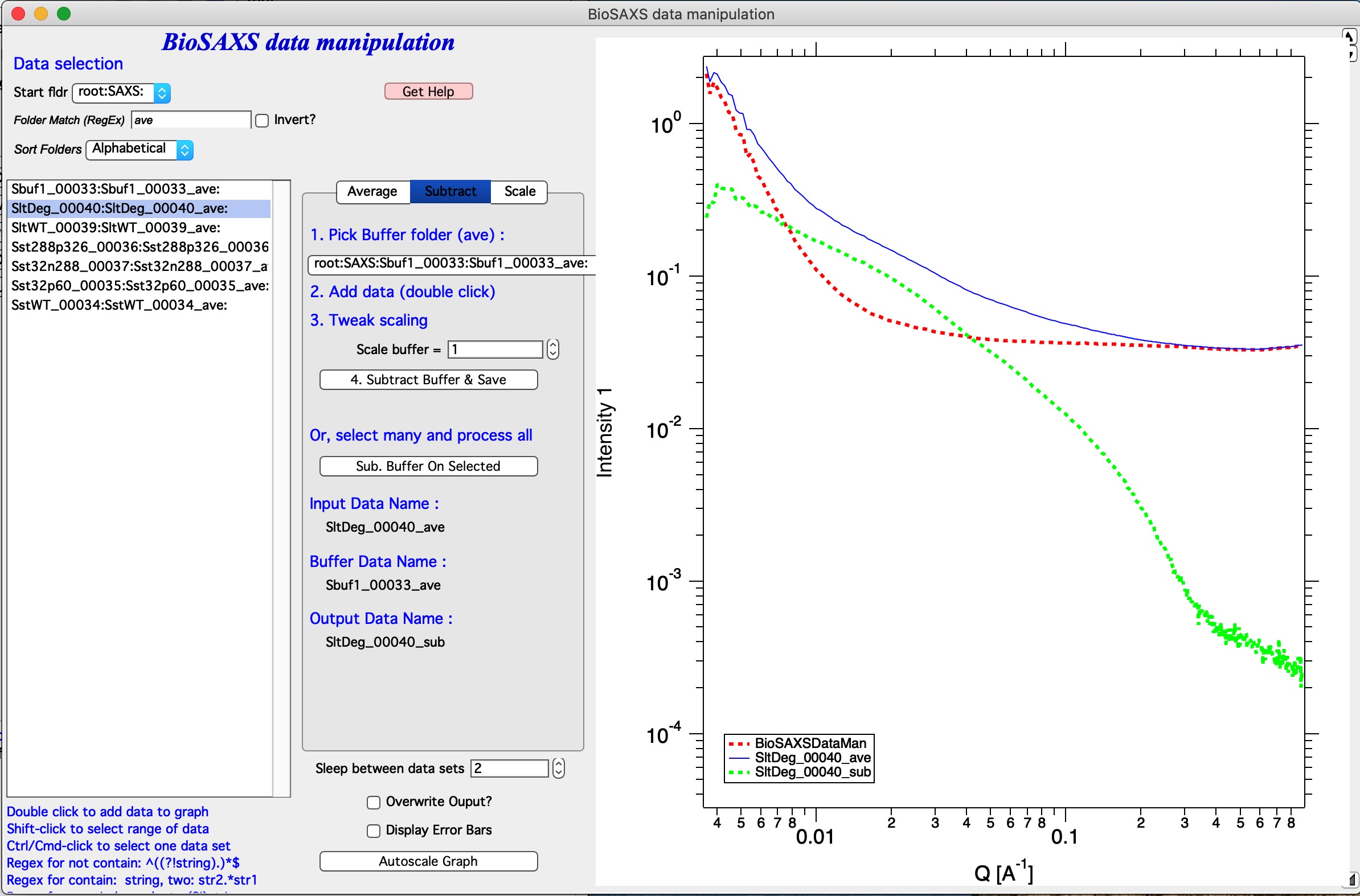
(Optional) tweak Scale Buffer value, if needed. Normally should be 1.
Hit 4. Subtract Buffer and Save button. Subtracted data (green line) will be added to the graph and data will be selected with _sub in name.
Now, if you have many data sets from which you need to subtract same buffer, with same scaling, you can run this in sequence. Select all data sets you want to process (Careful DO NOT select buffer measurement). Then use Sub. Buffer On Selected button and all data sets selected in the listbox will be processed in sequence.
Delay between the processing, which serves to let user review if the subtraction was OK, is controlled by Sleep between data set variable.
If you need to, you can check Overwrite Output? to prevent dialog if output data already exist.
NOTE: Code makes records in the history area:
Subtracted buffer from root:SAXS:SltWT_00039:SltWT_00039_ave:
Subtracted buffer from root:SAXS:Sst288p326_00036:Sst288p326_00036_ave:
Scale
If needed, user can scale more or less any data (Int-Q-Error) using Scale operation. It is useful for applying scaling factor (like absolute intensity scaling) to either averaged or subtracted data.
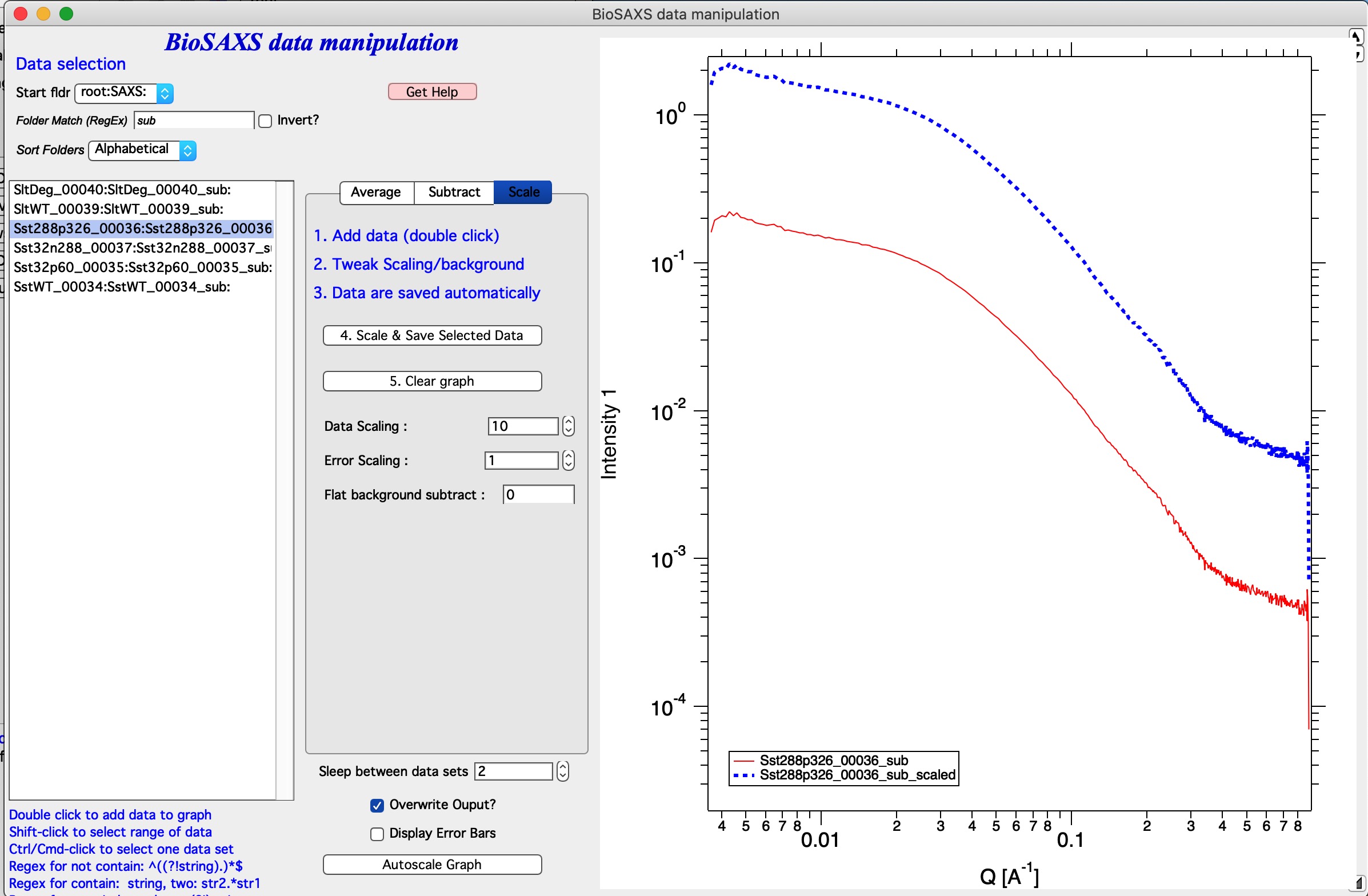
In the image I displayed only data which are subtracted (“sub” in the Folder match (RegEx)). I added data set into the graph and scaled by factor of 10. Code created a note in the history area:
Scaled data from root:SAXS:Sst288p326_00036:Sst288p326_00036_sub: and saved into new folder : root:SAXS:Sst288p326_00036:Sst288p326_00036_sub_scaled
Note, that the name changes by adding _scaled but leaves the _sub in there. From future use, these are subtracted_scaled data…
Concentration series extrapolation
This tool is used to subtract buffer from data measured with different concentrations, scale data by the concentration and extrapolate to concentration 0. Concentration and buffer scaling can be optimized to obtain optimal concentrations.
Requirement User needs at least three and at most five different concentration samples measured, reduced and normalized. User needs also buffers - either one buffer for each sample or same buffer for all samples. Reuse of buffers is allowed. User needs to have reasonable guess for concentration. For our test we have series of samples measured at 2, 4, and 8mg/ml concentrations and one buffer, same for all. The main GUI is below.
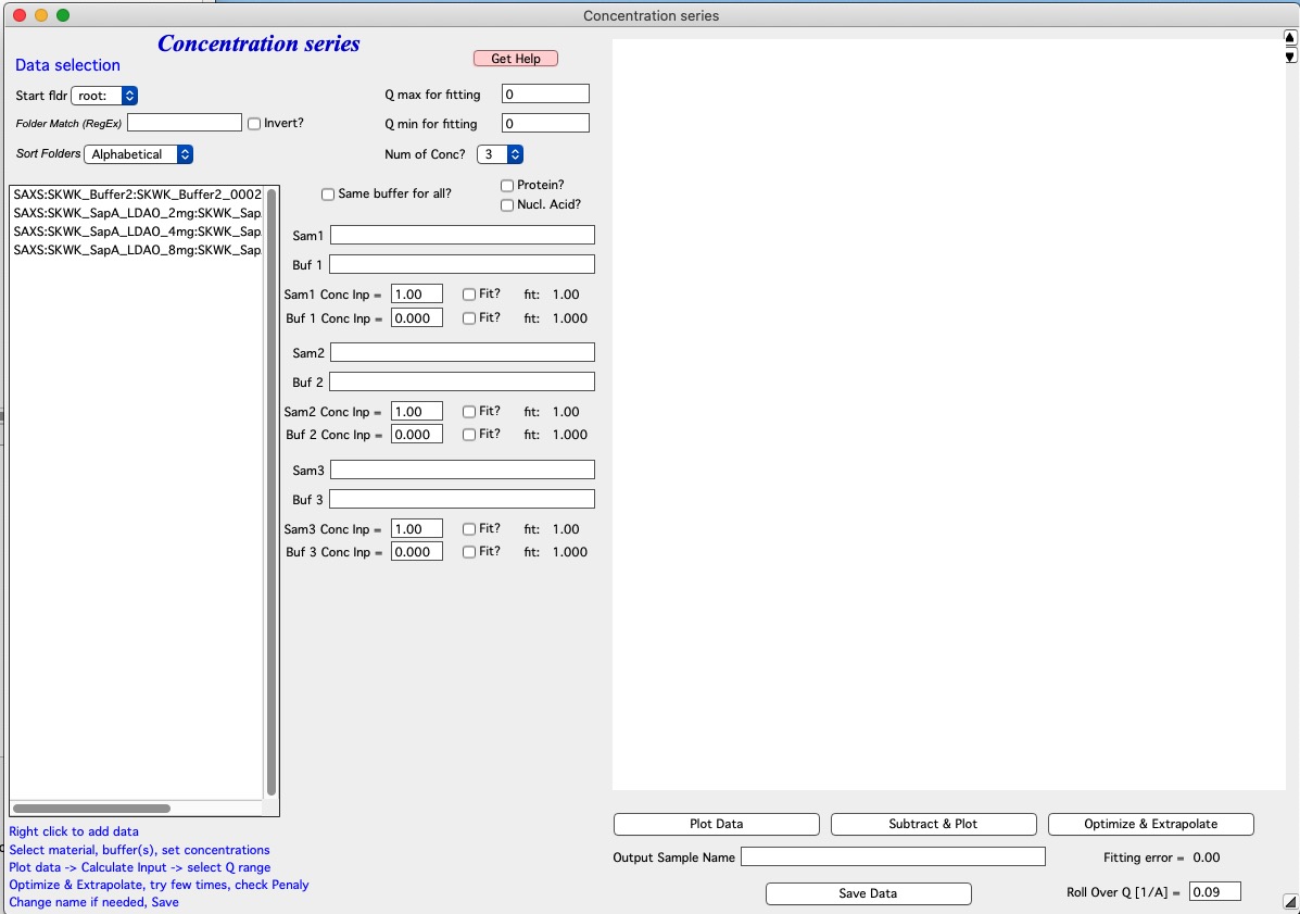
Use controls and selections on the left side of the panel to select samples. For example, in this case the names of samples end with avg, so we can reduce number fo samples displayed by adding avg in Folder Match field. We can also set Start folder etc.
Set Same buffer for all?
Select Number of Concentrations, select Protein? or Nucleic Acid? if appropriate.
Add samples in the Sample and Buffer Name fields. To add samples in the right fields, use right click menu when clicking on the sample name in the Listbox.
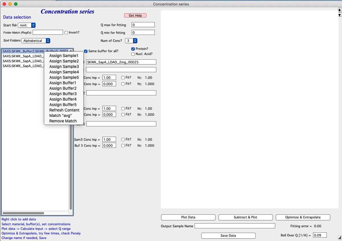
Next fill the Input Concentrations (SamX Conc Inp) in gm/ml. If you selected Protein? or Nucleic Acid? code will calculate estimate for buffer scaling based on empirical formula. Else, the value is left as is. In that case, make sure it is close to 1. When done, push Plot data.
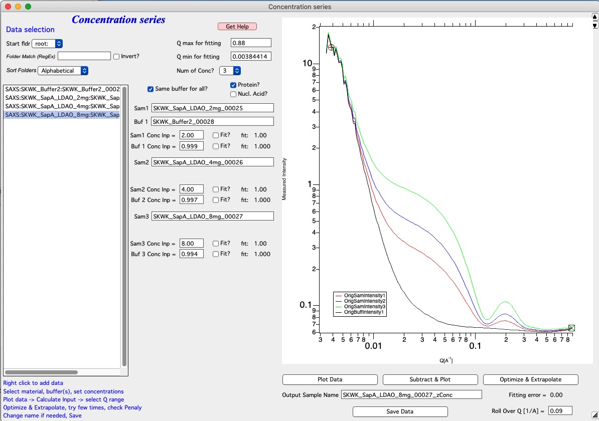
Next we need to select optimization/fitting conditions. Select using Fit? what you want to optimize. At least one concentration (suggested the highest one) must stay unchecked. The code will not allow the maximum concentration to be checked if user tries to select too many checkboxes. Next you need to also select Q range using cursors in which the data will be evaluated. When done, push button Subtract & Plot
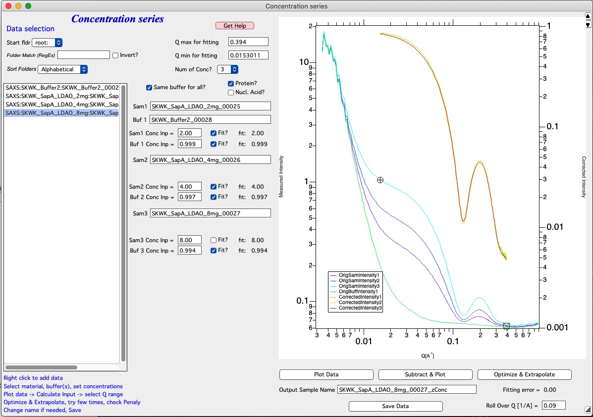
This graph now shows subtracted data plotted against right axis based on our estimates.
Next is Optimization/Fitting. If estimates look OK, use button Optimize and Extrapolate button to run optimization. Optimization takes some time, on my test data and fast Mac it takes about 6-10 seconds. After optimization is finished, code will extrapolate the intensity for cocentration 0. Th sis done using least square fitting of line for each Q point and extrapolating to 0 concentration. Since the data obtained this way at high-q values is usually quite noisy, data above Roll Over Q value are replaced with values for highest concentration measured (no extrapolation done).
Fitting Error Fitting error field provides information about final misfit of the data. Lower number is better fit. Sometimes there are few local minima which are close to global minimum and it may be worth trying few optimization runs to see, how low one can get with the Fitting error.
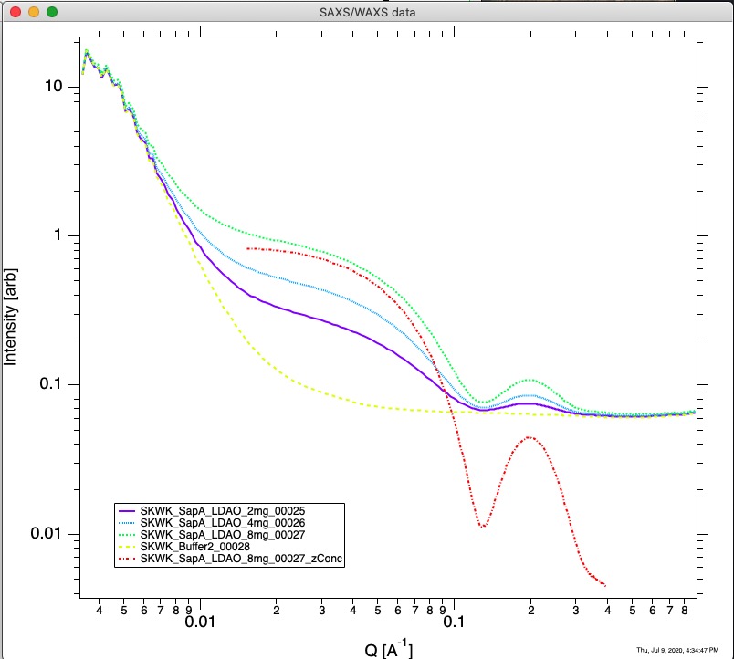
Save Data Pushing this button user can save these extrapolated data as zero concentration extrapolated data. By default code will set the Output Sample name field to name of the highest concetration sample. Code will remove “avg” string from the end (if present) and append “zConc” string. User can change the name as they want. NOTE: Output Sampe Name string has to be meaningful name for Igor Pro - single word starting with letter - little to no checking is done at this time.
Resulting new data, for rest of Irena are “QRS” data type with zConc appened to end of the name. NOTE: this zConc is appended by default, but user can change it - in which case user should remember what the name is. To be able to easily find them, set Folder Match String to zConc (it is case sensitive!). See image below to see resulting data obtained on this data set.
bioSAXS PDDF and Molecular weight
This chapter describes how to use bioSAXS PDDF and Molecular weight tool in Irena. This tool allows users to calculate Molecular weight using few different methods. It also allows users to utilize four different methods to generate PDDF from the SAXS data.
PDDF methods available and requirements
Following methods are implemented :
GNOM from ATSAS package. Users must have ATSAS (tested with version from February 2020; gnom -v returned : ATSAS 3.0.1 (r12314)).
autoGNOM - executable name is datGNOM from ATSAS package. Users must have ATSAS (tested with version from February 2020; datgnom -v returned : ATSAS 3.0.1 (r12314)).
Irena regularization method for PDDF (see Irena PDDF)
Moore method from Irena for PDDF (see Irena PDDF)
Molecular weight methods available and requirements
Following methods are implemented :
SAXSMoW2 method, reference: SAXSMoW 2.0: Online calculator of the molecular weight of proteins in dilute solution from experimental SAXS data measured on a relative scale, Vassili Piiadov, Evandro Ares de Araújo, Mario Oliveira Neto, Aldo Felix Craievich, and Igor Polikarpov, DOI: 10.1002/pro.3528, Protein Science 2019, Vol. 28, 454–463. This is method implemented in this tool: http://saxs.ifsc.usp.br
Rambo-Tainer methods, see Accurate assessment of mass, models and resolution by small-angle scattering, Robert P. Rambo and John A. Tainer, doi:10.1038/nature12070, Nature, Vol. 496, 2013.
Use of absolute intensity calibration and contrast estimate.
GUI description
The PDDF panel contains hopefully familiar left column data selection tools, see MultiData selection tools. This tool is set to handle ONLY QRS data type, if you need another data type (like USAXS), it can be added with some minor work. With these controls use selects one - or more - data sets for processing. Double click adds data set into the top graph so one can do analysis. It is possible to setup many data sets for analysis and run a sequence on them.
Next is middle column of controls, which contains tabbed interface. Details are later, but basically this area contains controls on data range selection, tabbed interface has the two methods used - PDDF and Molecular Weight analysis, and bellow the tabbed interface are results and how to handle the results.
The right hand side of the panel contains two graph areas. The top graph shows log-log Intensity vs Q vector data. Bottom shows appropriate data depending on tab selected - either PDDF graph or I(Q)*Q vs Q plot and the integration of this plot for Rambo-Tainer method.
Few other controls are around the edges of the panel and these are help controls which are useful for user operations, but are not primary operations.
Adding data
To add data, make appropriate starting folder selection and proper set Folder match (RegEx) if needed. Typically, you may want to show only subtracted data, like in example used here. In that case you put “sub” in this field and only data which have “sub” in name (results of buffer subtraction) will show. Double click will add data to graph.
When processing data sequentially, user need to select multiple data in the data selection Listbox. This can be done by holding down shift and selecting range or holding down ctrl/cmd and clicking on specific data names. Users also should use Sort Folders to make sure data are processed in meaningful sequence. This makes it easier to plot results, as they are already sorted according to whatever user needs.
PDDF controls
The main control here is Method checkboxes - four options are available, default is GNOM, optional are autoGNOM, Irena Regularization, and Moore. Each has its own selection fo controls. which are listed below:
Rmin==0? this is applicable only to GNOM and forces GNOM to set PDDF so at Rmin (=0 A) the PDDF=0. Default is checked.
Rmax==0? this is applicable to GNOM and forces GNOM to set PDDF=0 at Dmax value. Default is checked.
Alfa in this is applicable only to GNOM and is input value for alfa. If set to 0 (default), this command is skipped and GNOM is run without setting starting alfa condition.
R pnts this is applicable to most methods, sets real space number of bins. If =0 this parameter is not passed to programs which allow it (GNOM or autoGNOM). Irena tools require this parameter and default is 100 for those. Default is 0 unless Regularization or Moore is selected, then it is 100.
Dmax estimate This parameter is applicable for all methods. User needs to set meaningful value. Default is 30, which is likely wrong for any sample.
Num Func This parameter is applicable only to Moore method. Default is 100.
Det Num Functions? This checkbox is applicable only to Moore method. Default is unchecked.
Fit Max Size This checkbox is applicable only to Moore method. Default is checked.
Molecular weight controls
These calculations need sometimes either density or scattering length of material studied. The code has these values for Protein and Nucleic Acid. User needs to select correct material using the checkboxes Protein and Nucleic Acid.
Fit Rg and Calculate MW button will fit Guinier law on the data - twice. One without flat background and second time with the flat background. This way code gets Reciprocal fitting values and the background used in this method. User needs to set cursors in the graph since fitting of the Guinier law is done between the cursors.
Qmax 8/Rg this is for SAXSMoW and Rambo-Tainer methods, sets Qmax for integration to 8/Rg (formula 7 in SAXSMoW paper).
Qmax I(0)/200 this is for SAXSMoW2 and Rambo-Tainer methods, sets Qmax for integration to Q when I(Q) = I(0)/200 (see SAXSMoW paper formula 8).
Qmax user can put any Qmax here. Be careful…
Auto find background Applicable only to Rambo-Tainer method. In this method - for samples with poorly subtracted buffer - Qmax and background cause large uncertainties. By fitting flat background code can estimate the flat background Which may improve stability of the results. Checking this checkbox uses the fitted flat background for subtraction.
Subtract background Applicable only to Rambo-Tainer method. Will actually subtract the background for analysis.
Flat background this is value which will be subtracted. User can change as needed. See later.
C [mg/ml] this is concentration, which is needed for method using GNOM output results (Real space results) which relies on absolute calibration of the data. In this case code needs to know contrast (provided by choice between Protein and Nucleic acid), concentration, and absolute intensity.
Mol Weight Results
In this are are summarized results from both tabs. Results obtained from PDDF are called “Real Space results” while results obtained using Intensity fitting are “Reciprocal space results”.
Reciprocal space results Are obtained from Guinier fit to the data (button on the Mol Weight tab). First we present fitting results and partial data: Rg, I(0), and Porod volume. Next are Molecular weights calculated based on SAXSMoW method and Rambo-Tainer method.
Real Space results. These depends on number of conditions. First, all are available ONLY when user uses GNOM or autoGNOM. Absolute intensity estimate MW depends on, well, absolute intensity calibration of the data. Again, we present first Porod volume, Rg, and I(0). Then SAXSMoW method calculating the Molecular weight, but this time using GNOM fitted intensity to the data. And finally, the estimate using GNOM parameters and depending on absolute intensity and concentration.
Save results controls
Folder selecting this checkbox will save results of the fit into the folder with data. This way one can probe the results later with Metadata Browser or plot them with one of the Irena Plotting tools. Number of waves are saved which contain PDDF, Intensity fit etc. Hopefully with meaningful names. If user used GNOM or autoGNOM, code will also save whole GNOM out file as text wave in the folder.
Notebook selecting this checkbox will save results in Igor Notebook record. Results are summarized and graphs inserted.
Waves selecting this checkbox will save results in waves in folder with specific name. These can then be plotted or put in table by users. Meaningful names should be easy to understand.
GNOM out selecting this checkbox will be useful ONLY, if GNOM or autoGNOM is used. If checked, code will create folder outside Igor, on user hard drive, in the folder where current Igor experiment is located. Lets assume current Igor experiment is called “MyTestAnalysis” and is located in MyDocuments folder. PDDF code will create a new folder called “MyTestAnalysis_GNOM_OUT” folder there and place in this folder copies of GNOM.out files which were generated during analysis. Files are named by using data names in Igor, e.g. BSA_SASDA32_sub data will have BSA_SASDA32_sub.out in that location. Same name files in export location are overwritten.
Save PDDF results This button will save results as instructed by the checkbox settings. Selecting checkboxes themselves does nothing until this button is pressed.
Open Table and Notebook will open the table with wave and Notebook, if such data were saved by checkbox selection.
Delete results waves will remove the folder with results and kill the table.
Overwrite output overwrites output data so user does not have to answer questions when data are already found.
Sleep between sets this is setting in seconds, when running sequence of GNOM fits, this will force code to sleep between the samples to give user time to inspect the fits and note if some sample need s to be revised later. Default is 0.
Display error bars Error bars are useful but can be distracting. User has choice to see or not see them.
Autoscale graph - graphs embedded in panels do not react to usual autoscale command (ctrl/cmd-A) in Igor, so one either has to right click and select Autoscale or use this button.
How to fit Molecular weight
This will walk users through the Molecular weight fitting. As noted above, there are four different method, the most used one will be likely using GNOM which is available as part of ATSAS package. This one will be used for this example, the other methods have minor differences in controls which will be only marginally mentioned.
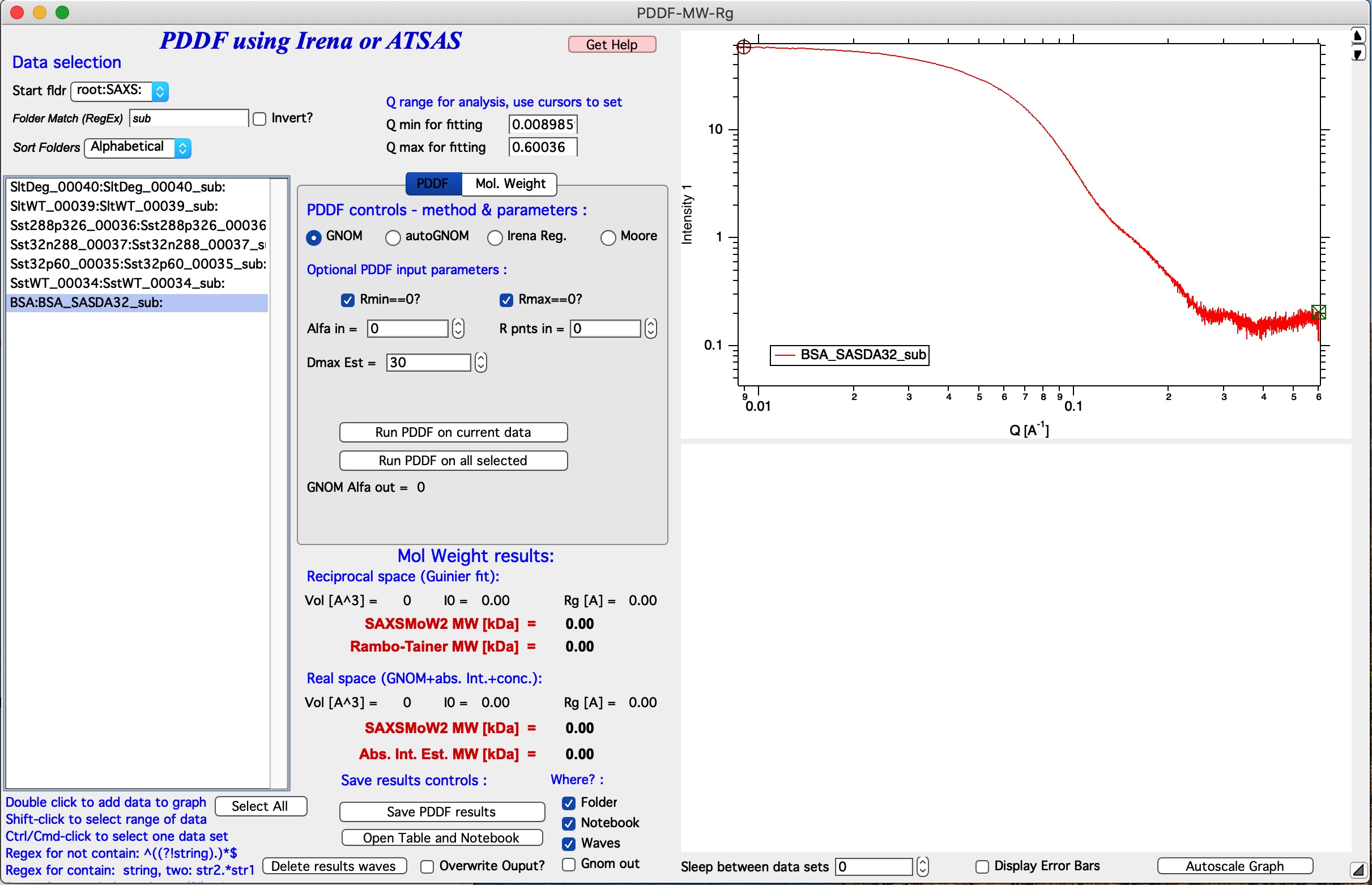
Add data in the graph by double clicking on the data, in our example we use BSA data available here: http://saxs.ifsc.usp.br/SASDA32.dat which are used as example for SAXSMoW tool: http://saxs.ifsc.usp.br. Warning: when importing these data, convert Q unit from 1/nm to 1/Angstrom, these data use 1/nm for Q.
Go to Tab for Mol. Weight. Select with cursors data from Q around 0.02 to 0.1. NOTE: circle cursor A must be at low-Q, square cursor B must be at high-Q. Hit button Fit Rg and calculate MW.
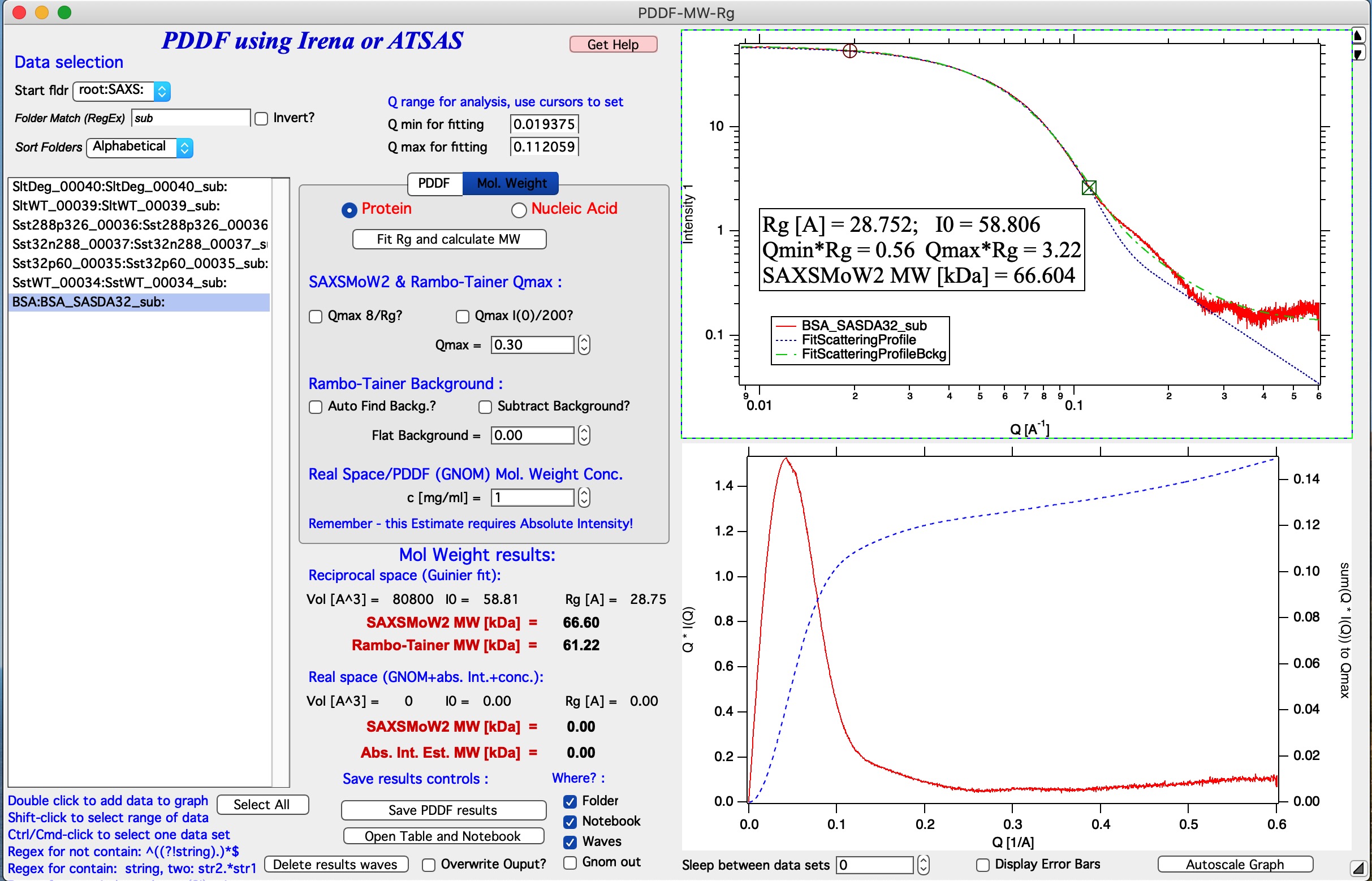
Now, we have a good fit and therefore good values for Rg and I(0). Now we need to make sure the right Q range is used for SAXSMoW method. Check Qmax 8/Rg and values should update. This fixed Qmax for both methods used here to about 0.28 [1/A]. Users can make different choices here and discussion on what is right is not part of this manual.
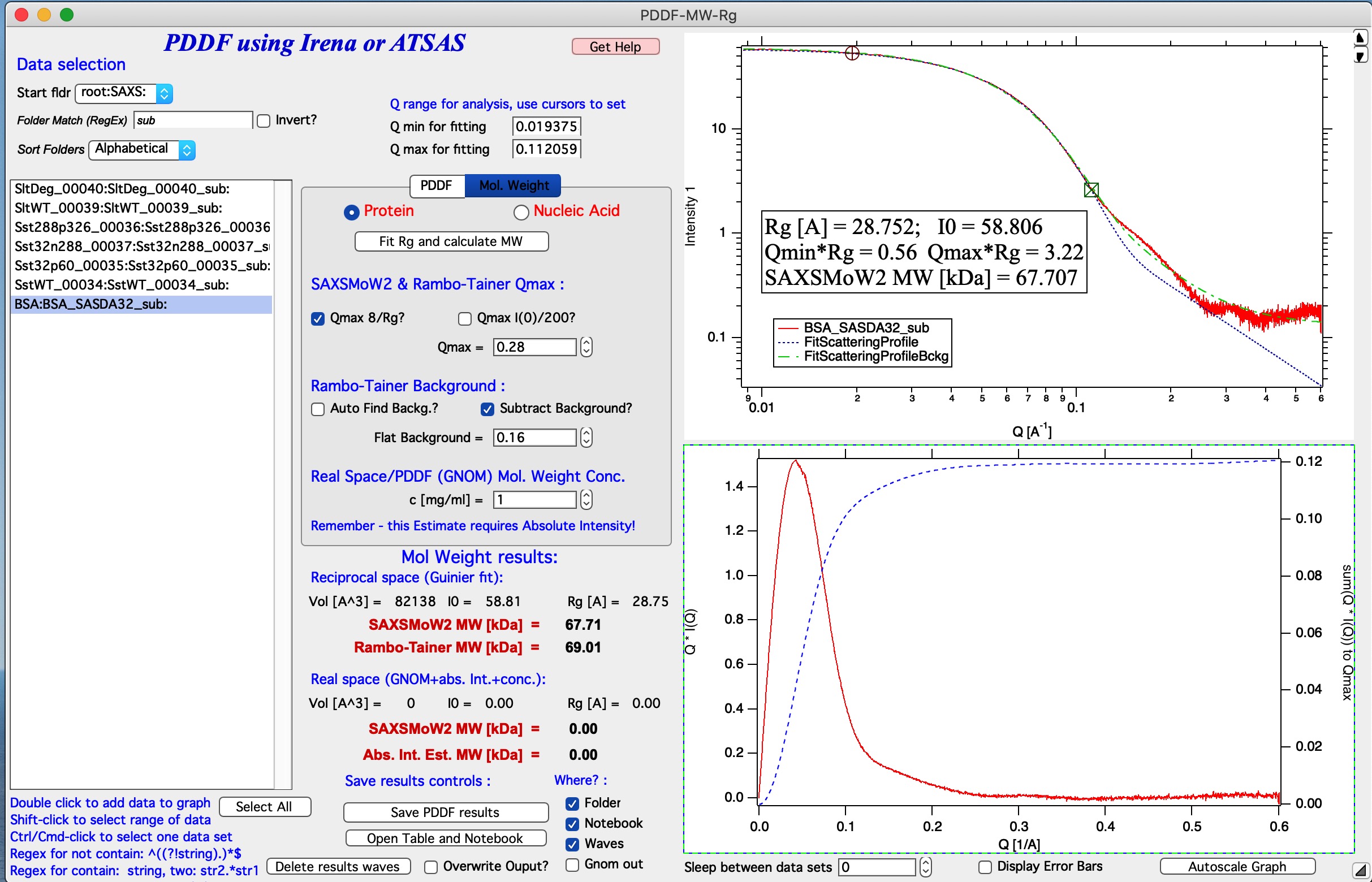
If you look on the blue curve in the bottom graph, you can see, that the integration of Q*I(Q) does not reach plateau. It should in order for Rambo-Tainer method to work as this integration is effectively version of invariant. This is due to poor subtraction of buffer for this sample. Check The Autofind Backg? checkbox and re run the Fit Rg and calculate MW.
Now we have value in the Flat background which code found as first guess of the flat background in this measurement. Check the Subtract Background? checkbox. This changes the blue curve in lower image which now nearly reaches plateau. Tweaking the Flat background to about 0.16 will make the intergation of the Q*I(Q) reach plateau at around Q=0.25 and integration to any value above that is returning pretty much same value. This suggest we subtracted proper background -assuming the differences are due to incorrect buffer subtraction and that can be approximated as flat background…
Now, this suggests, that we now have reasonable solution and obtained two approximations of Molecular weight.
How to fit PDDF
Now we will fit PDDF using GNOM to these data. Note, that the Rg is around 30A, suggesting we need to assume max size around 70-90A. Switch to PDDF tab, this will clear the bottom graph.
Select radiobutton GNOM if it is not selected. Check the checboxes Rmin==0 and Rmax==0 set Alfa in = 0 and R pnts in = 0, set Dmax Est = 90.
Select Q range for fitting. Only data between cursors will be exported in dat file for GNOM. Data from Q=0.013 to Q=0.13 are suitable for fitting, even though it does not seem to matter too much on this very good sample.
Now push button Run PDDF on current data. When running first time you will get a dialog to find where GNOM executable file is located. Read the instructions and hit button OK.
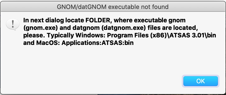
In the next system dialog, locate Folder (directory) in ATSAS folder called “bin” and select that directory. This is where the binaries for gnom and autognom are.
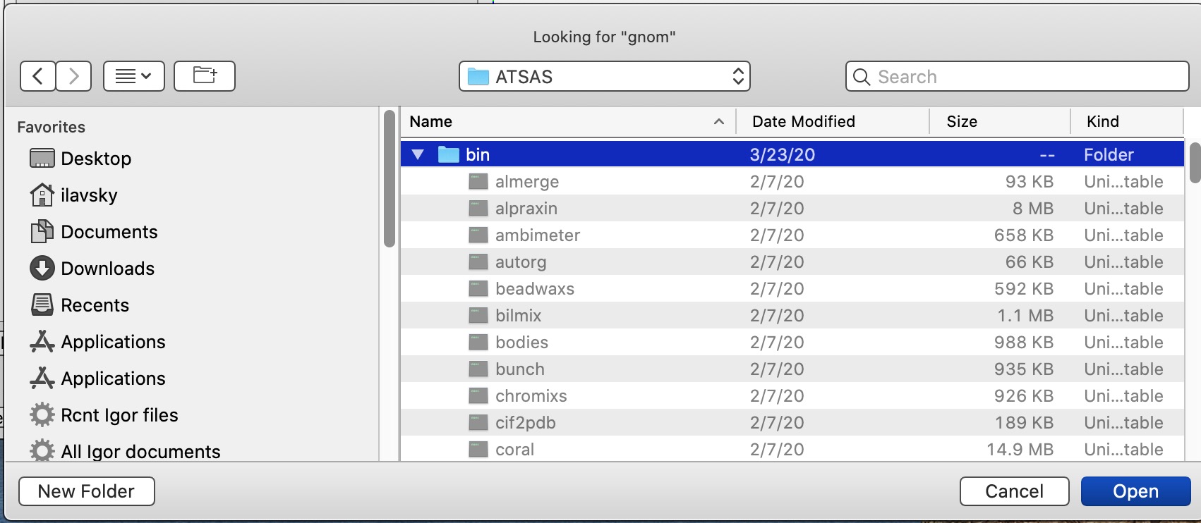
Code will write out dat file as input for gnom in system provided temp directory and run gnom with appropriate command flags as selected in the GUI. It will wait for gnom to finish and read the OUT file in. It will then run through some calculations and present the results.
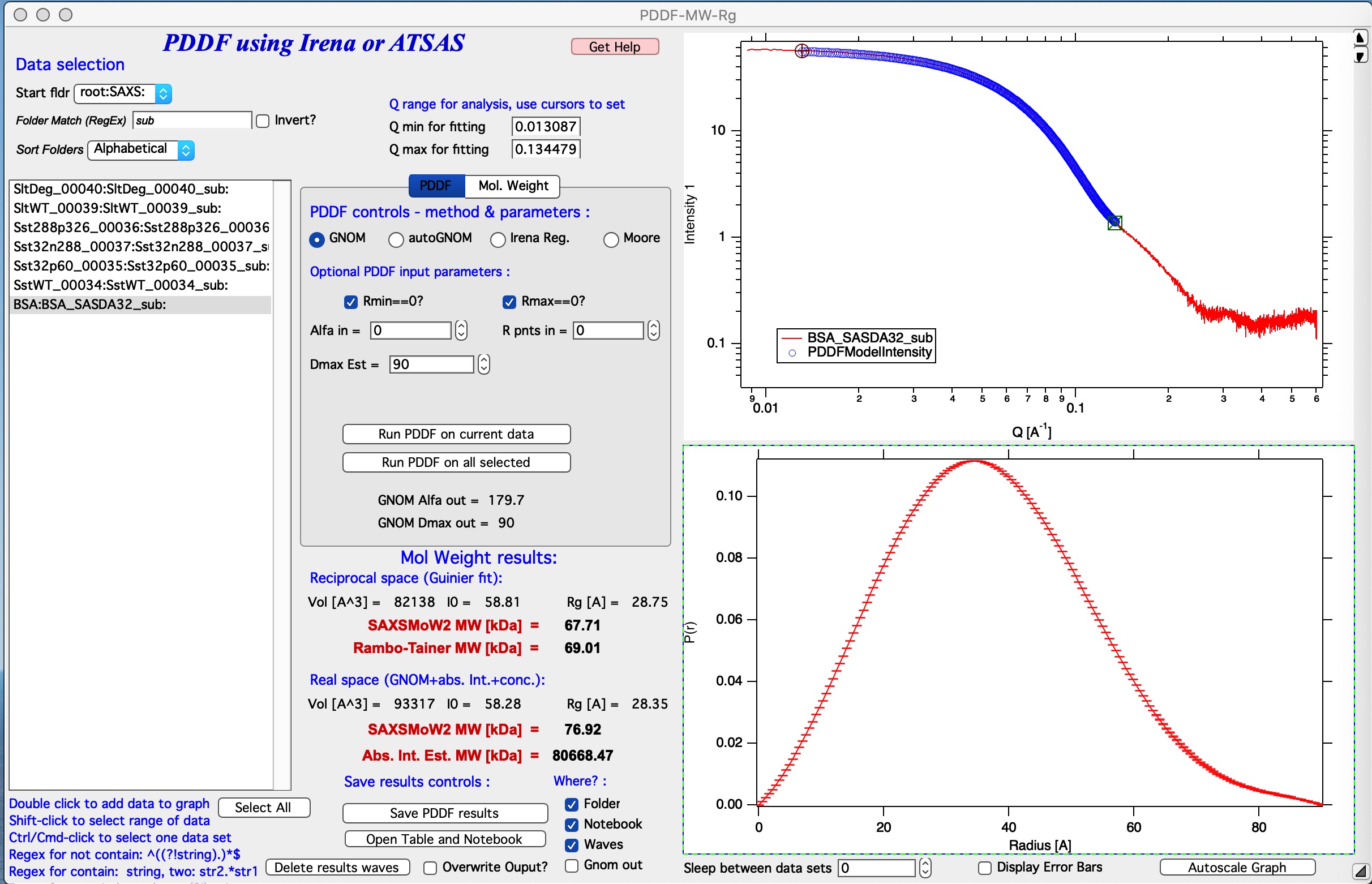
Description of results
Running GNOM or autoGNOM provides following results: 1. PDDF displayed in the graph (and saved as needed in notebook or folder) 2. Fit to the data displayed in the log-log Int/Q plot. The blue points represent GNOM fitted results. 3. GNOM calculated I(0), Rg, and Porod volume, these are called Real Space results. 4. Using GNOM calculated Intensity/Q model code will use SAXSMoW2 method to calculate Molecular weight. This is called Real space SAXSMoW2 MW.
Save the results
Here are examples how the data are saved, in pictures…
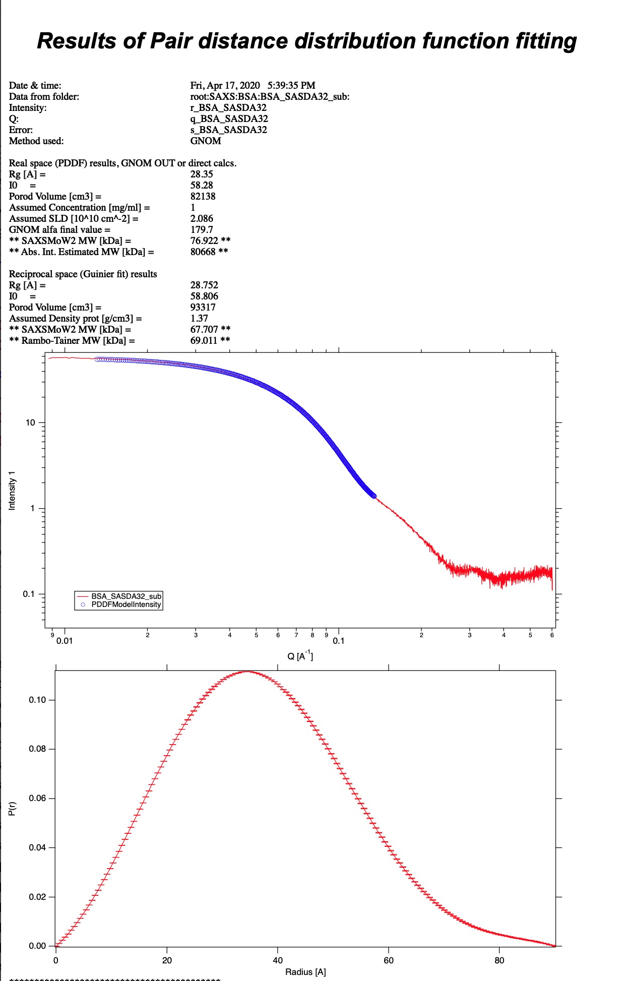
Image above shows record in Notebook.
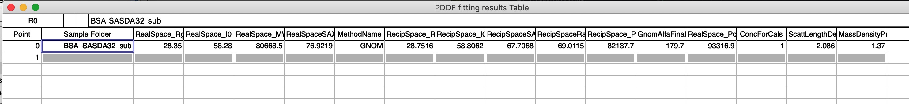
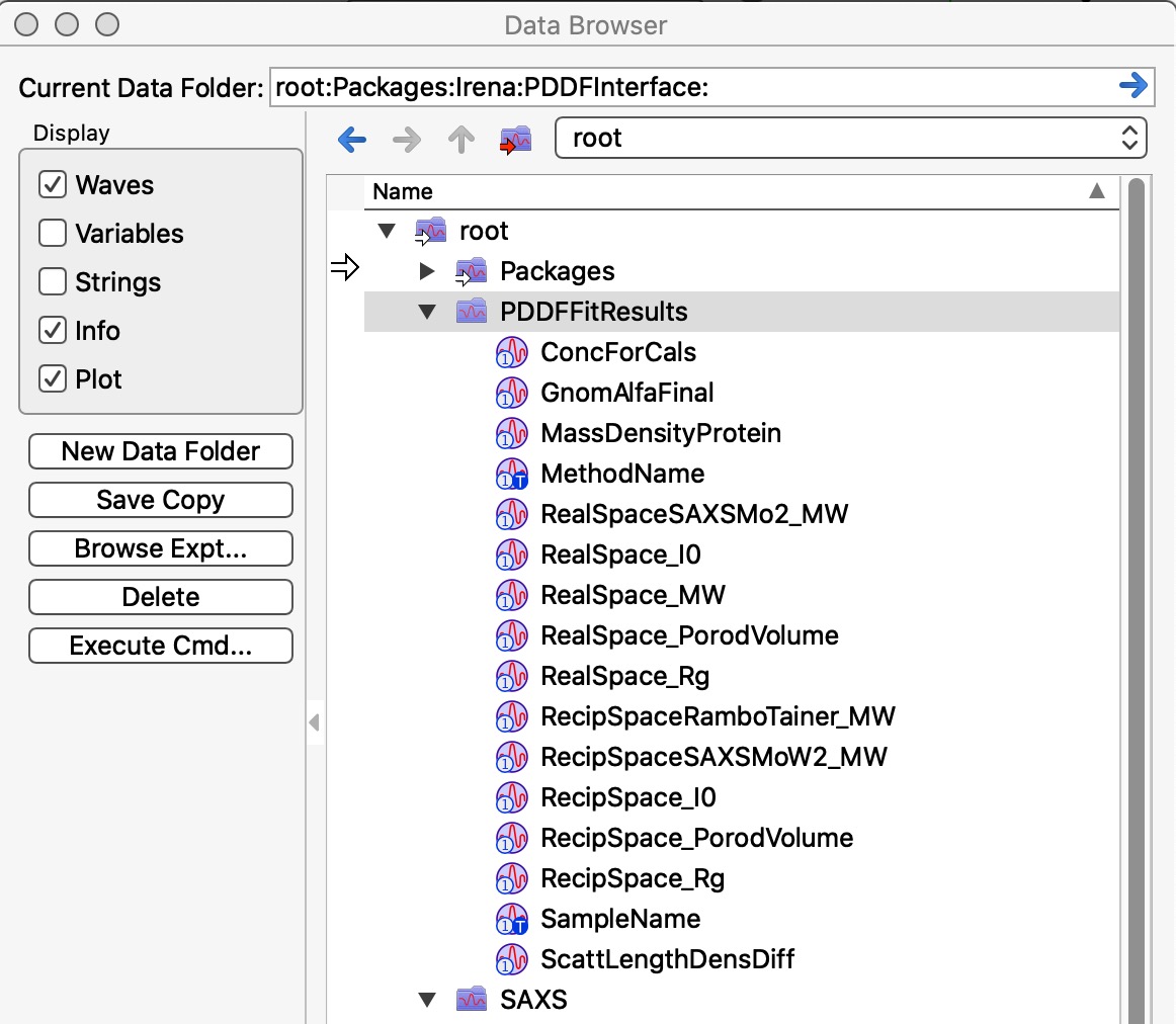
The two images above show record created in Igor experiment. A folder called root:PDDFFitResults will be created, waves which can be seen in the image are created and every time user saves new results a new line is added to each of the waves. These waves are used to create the table seen in the image above. Old data are not overwritten, unless used deletes them all using the button on the panel. Therefore, same data set can be in the table many times.
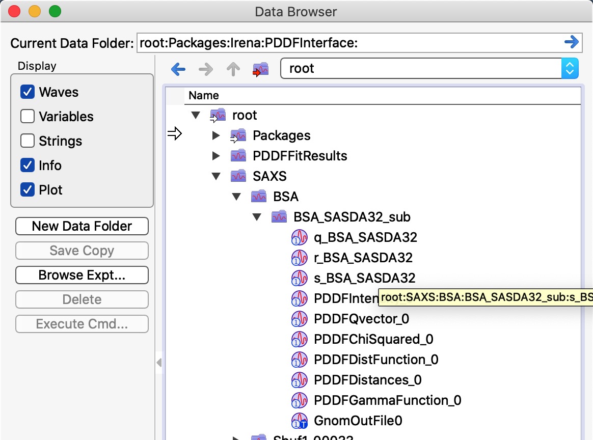
Image shows which wave are saved in Data folder with the data. Multiple “generations” can be saved, data are not over written. User needs to delete them manually, if necessary. These are seen by rest of irena as Irena results.
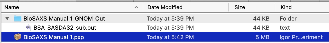
And finally, this is GNOM out file saved where this experiment called “BioSAXS manual 1.pxp” is located. New folder is created and all OUT files are saved there. Out file of the same name will be overwritten. User is warned by dialog which asks for permission to overwrite the out file.