System specific models
This tool provides a GUI for analytical models applicable to specific microstructures:
Debye-Bueche — structural inhomogeneities in gels. https://onlinelibrary.wiley.com/iucr/itc/Ha/ch5o8v0001/sec5o8o3o1o4/
Treubner-Strey — small-angle diffraction.
Ciccariello-Benedetti — coated smooth surfaces.
Hermans, Modified Hermans, and Unified Born-Green — polymer lamellar structures. See: https://doi.org/10.1016/j.polymer.2021.124281
Most models can be combined with a low-Q single Unified level. Only one model can be active for any dataset at a time.
For the Unified level controls, see the Unified Fit documentation. RgCO can be linked to the best-guess parameter combination from Debye-Bueche, Treubner-Strey, and other models. Residuals are plotted as dots in the graph.
Tool overview and use
The tool is demonstrated below using the Debye-Bueche model, but the workflow is the same for all models. The tool uses the multi-sample data selection interface also used by the BioSAXS tools and the Multi-Sample Plotting tool. See Multi Data selection.
The top section contains controls for selecting data type (USAXS or QRS), slit smearing vs desmearing for USAXS data, and a folder match string (regular expressions supported — see the hint at the bottom of the panel).
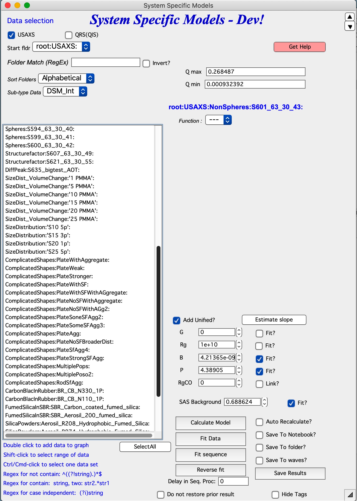
Controls
Adding data: Double-click a dataset in the listbox to load it and create a log-log plot. The blue text above the Model pull-down menu shows the currently active dataset.
Model: Select a model from the pull-down menu. The area below the menu populates with controls for that model. Details are in the model-specific sections below.
Unified Fit: Controls appear when the “Add Unified?” checkbox is enabled. Five parameters are available: G, Rg, P, B, and RgCO. RgCO is critically important: when linked, it terminates the Unified level scattering at the scale of the model features, indicating that the Unified level and model scattering arise from the same phase. If the Unified level scatters from a separate phase (e.g., surface scratches), set RgCO to 0 and do not link it. “Estimate slope” fits P and B to the data range selected by cursors.
Background: Flat background, constant across all Q values. Can be fitted.
Controls and buttons:
“Calculate model” — computes the model with current parameters. “Auto Recalculate?” forces recalculation after every parameter change.
“Fit data” — fits the currently loaded dataset. Only parameters with “Fit?” checked are refined. Verify that fitting parameter ranges are set appropriately.
“Fit sequence” — fits all datasets selected in the listbox, top to bottom. Sort the list appropriately before running.
“Revert fit” — restores parameters to their pre-fit values.
“Save results” — saves model output. What is saved depends on the checkboxes:
“Save to Notebook?” — appends a results summary and plot to the Results notebook.
“Save to folder” — saves model intensity and Q waves to the source data folder. Saved results can be reloaded later: if a matching solution is found in the folder, the tool offers to restore those parameters.
“Save to waves” — creates a results folder (e.g.,
root:DebyeBuecheResults:) and saves individual parameter waves there in processing order. Useful for plotting parameter trends across a dataset series.
“Delay in Seq. Proc.” — wait time between sequential fits; allows visual inspection and note-taking.
“Do not restore prior results” — suppresses the offer to reload saved parameters when loading data.
“Hide tags” — removes parameter tags from the graph.
Models
Debye-Bueche model for gels
The Debye-Bueche model (https://onlinelibrary.wiley.com/iucr/itc/Ha/ch5o8v0001/sec5o8o3o1o4/) is implemented as:
where \(K = 8 \pi ^2 \lambda^{-4}\), ξ is the correlation length, and ε is the mean-square fluctuation parameter.
The model also supports a low-Q power-law slope and a flat SAS background, both optionally fitted.
From Hammouda (NIST): The Debye-Bueche model describes scattering from phase-separated (two-phase) systems with correlations characterized by an e-folding length ξ. The pair correlation function (Debye-Bueche, 1949):
Scattering cross section:
where the prefactor is:
The Debye-Bueche model is a limiting case of the Teubner-Strey model for very large d-spacing (d >> ξ).
Typical plot:
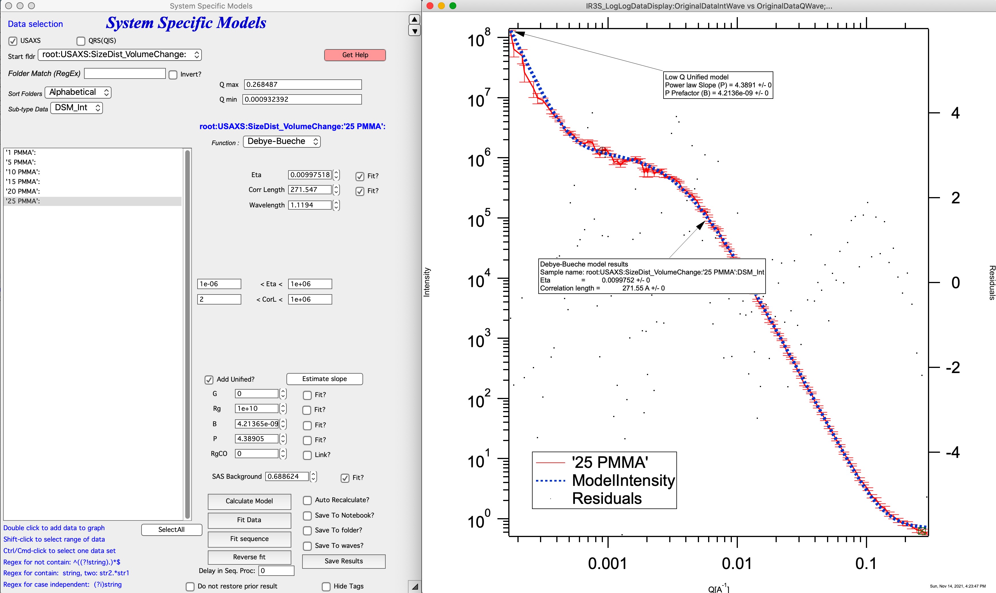
This example uses Eta and Corr length, with wavelength read from the data header (or set manually if not available). The power-law Unified level is applied here (see Unified Fit documentation for details on using G = 0 and Rg = 1010).
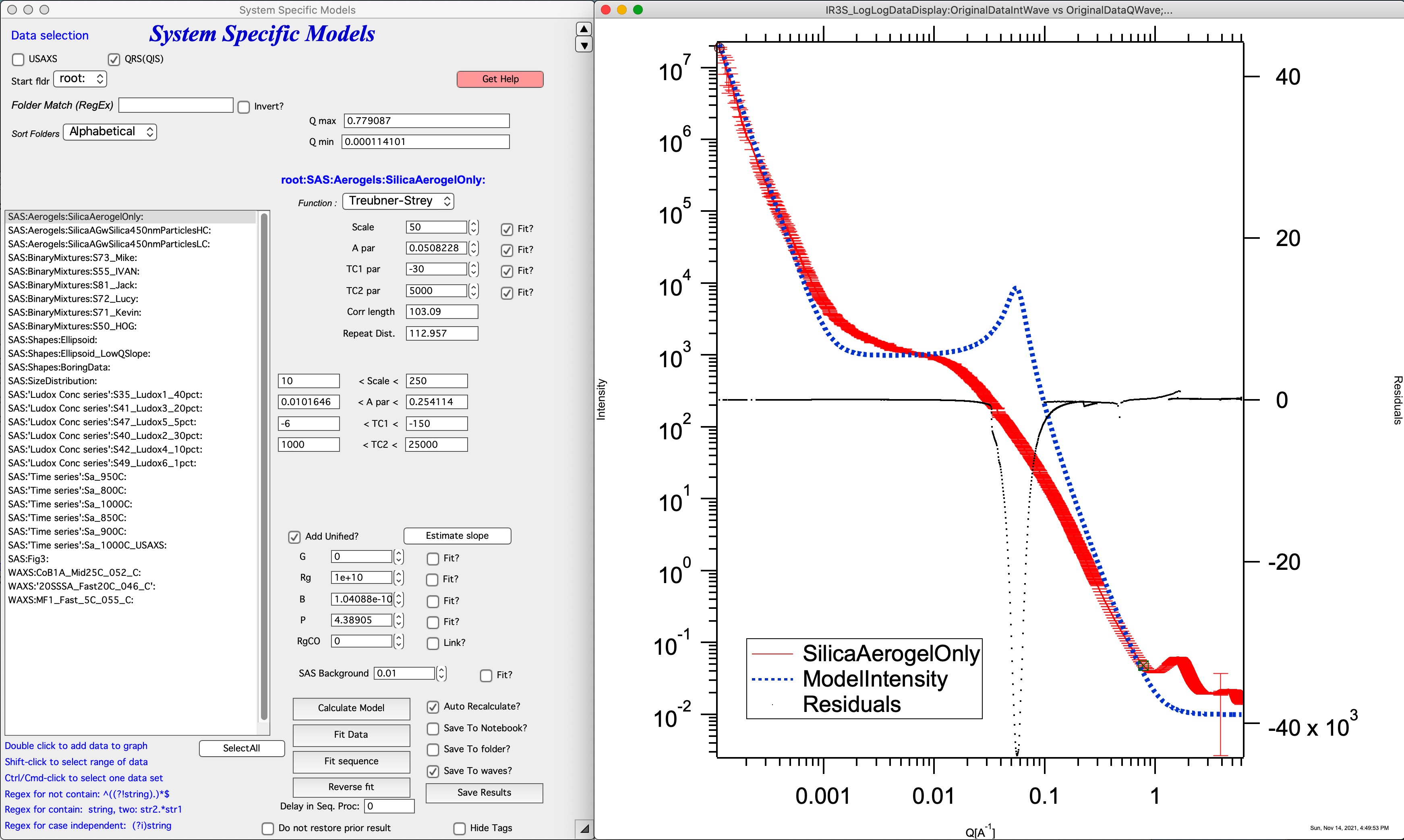
Treubner-Strey for small-angle diffraction
References:
Teubner, M.; Strey, R. J. Chem. Phys. 1987, 87, 3195. https://doi.org/10.1063/1.453006
Schubert, K-V.; Strey, R.; Kline, S. R.; Kaler, E. W. J. Chem. Phys. 1994, 101, 5343. https://doi.org/10.1063/1.467387
More recent description: https://doi.org/10.1016/j.polymer.2004.08.033
The code is adapted from the NIST SANS package:
where A, C1, and C2 are theory parameters and TS is a scaling factor. Correlation length ξ and repeat distance d:
Only TS, A, C1, and C2 are user-controlled.
Ciccariello-Benedetti model for coated smooth surfaces
References:
Benedetti, A.; Ciccariello, S. J. Appl. Cryst. (1994) 27, 249–256.
Pikus, S.; Kobylas, E.; Ciccariello, S. J. Appl. Cryst. (2003) 36, 744–748. https://doi.org/10.1107/S0021889803000244
This model assumes a constant-thickness, constant-SLD layer on the surfaces of a porous medium, where the layer is always parallel to the underlying surface. The Porod Q-4 slope is modified by an oscillatory term from which the film thickness and contrast can be extracted.
Note
Discrepancies have been observed between results using finite slit length (Irena’s internal smearing routines) and infinite slit-length approximations. Results depend on the assumed slit length.
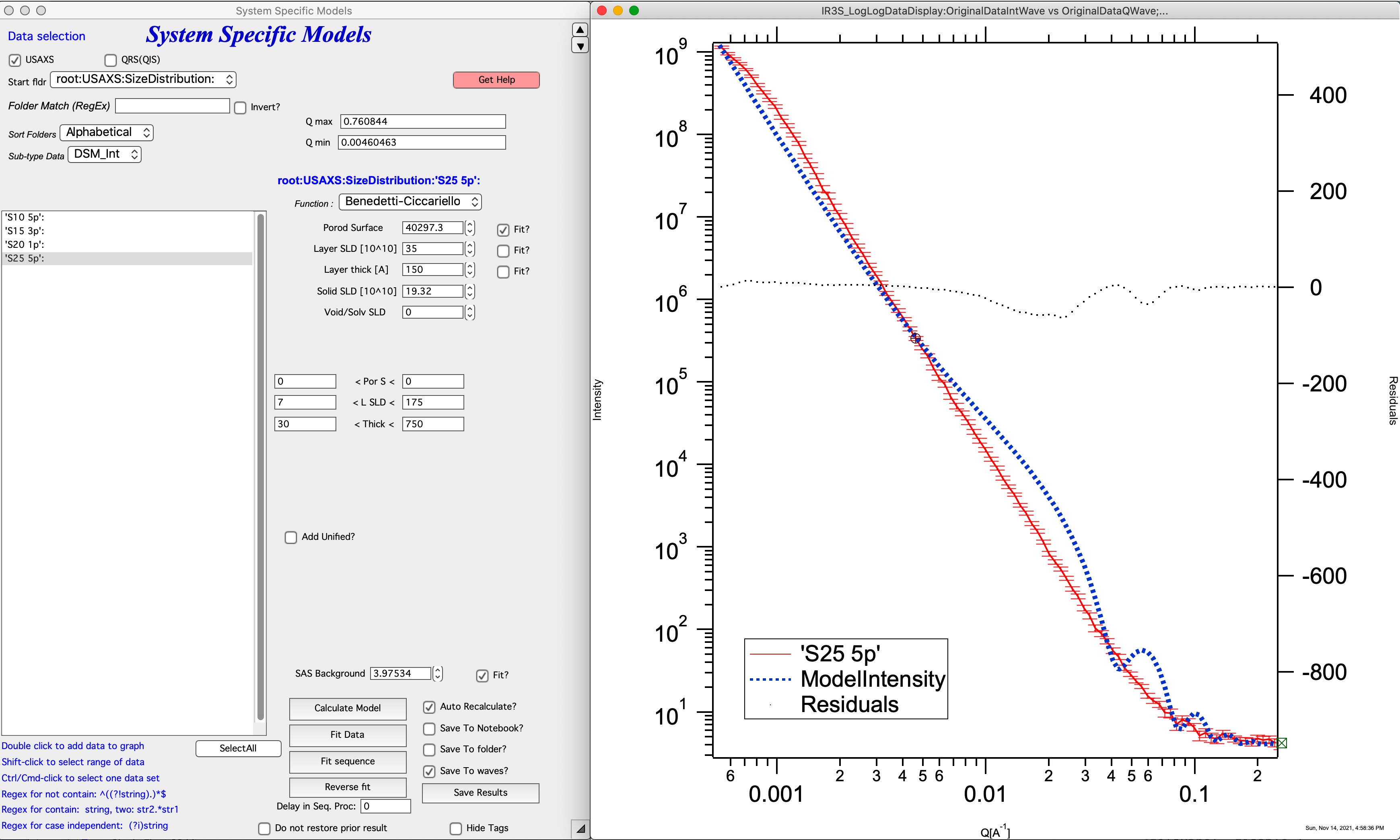
Fitted parameters:
Porod specific surface area — area of the solid/void or solid/solvent interface (without the layer).
Layer SLD — scattering length density of the layer.
Layer thickness — in Å.
Fixed parameters (known a priori):
Solid SLD — scattering length density of the solid phase.
Void/solvent SLD — typically 0 for air.
Also set the SAS background and fitting limits as usual. Combining this model with a Unified level is generally not physically meaningful.
Hermans model for lamellar systems
The Hermans model assumes independent normal distributions for the crystalline and amorphous regions of lamellae, with infinitely wide, perfectly aligned, regularly spaced sheets. Five parameters: mean crystalline thickness (tL), its standard deviation (σL), mean amorphous thickness (ta), its standard deviation (σa), and a Porod prefactor for surface scattering (B1).
The model describes the Porod surface scattering region, the Guinier region for lamellar thickness, the structure factor for lamellar stacking, and the 2D scaling regime for infinite-width lamellae. It does not describe lateral extent or higher-order structures (fibrous stacks, spherulites).
For USAXS measurements: the model assumption of perfectly lamellar sheets produces a −2 power-law slope at low Q.
For details: https://doi.org/10.1016/j.polymer.2021.124281
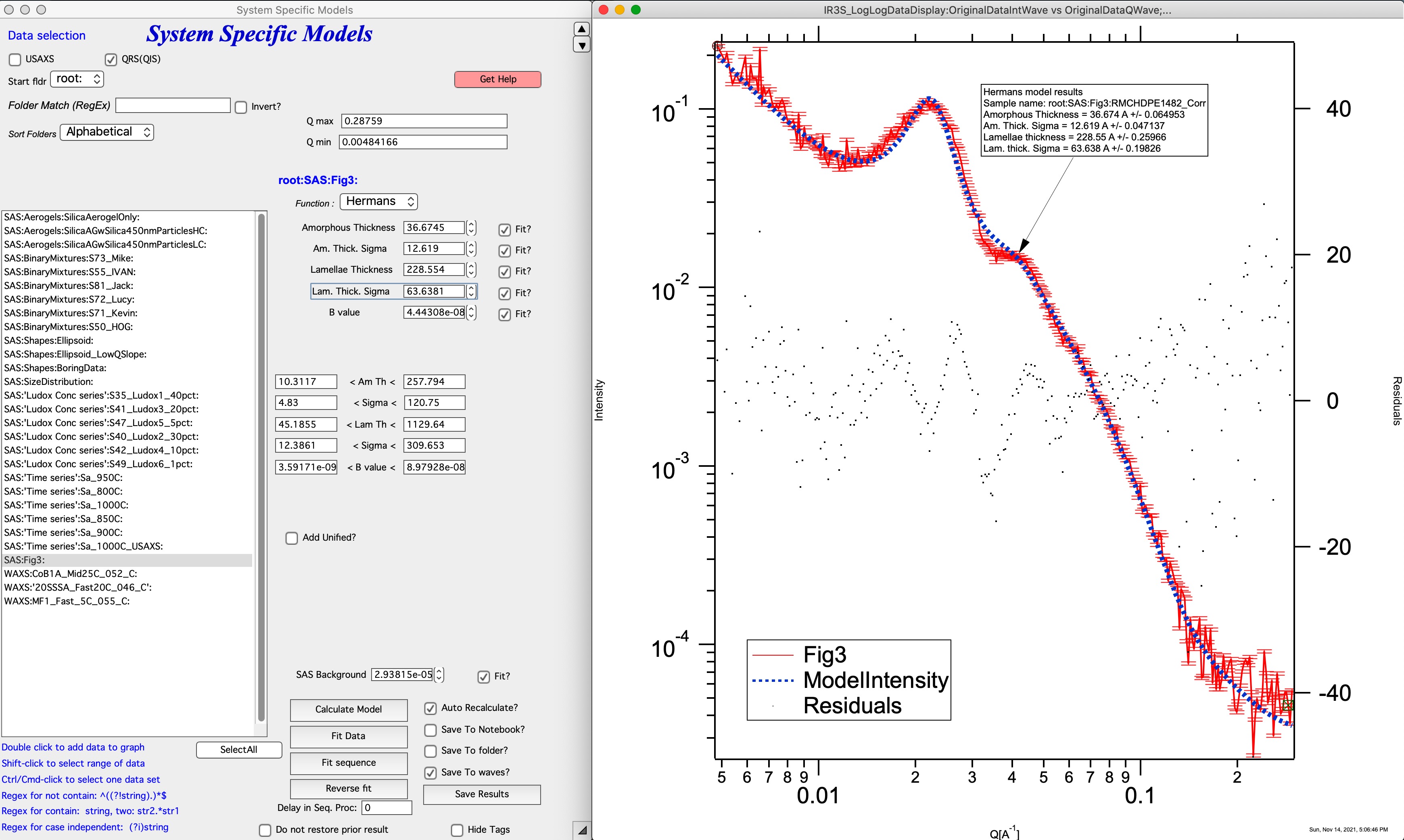
Note: this model has many parameters and solution uniqueness may be limited.
Modified Hermans model for lamellar systems
Like the Hermans model, but adds Unified function terms (Rg2, G2) to describe higher-order structures associated with lamellar stacks. Total parameters: seven when limited to lamellar width.
For details: https://doi.org/10.1016/j.polymer.2021.124281
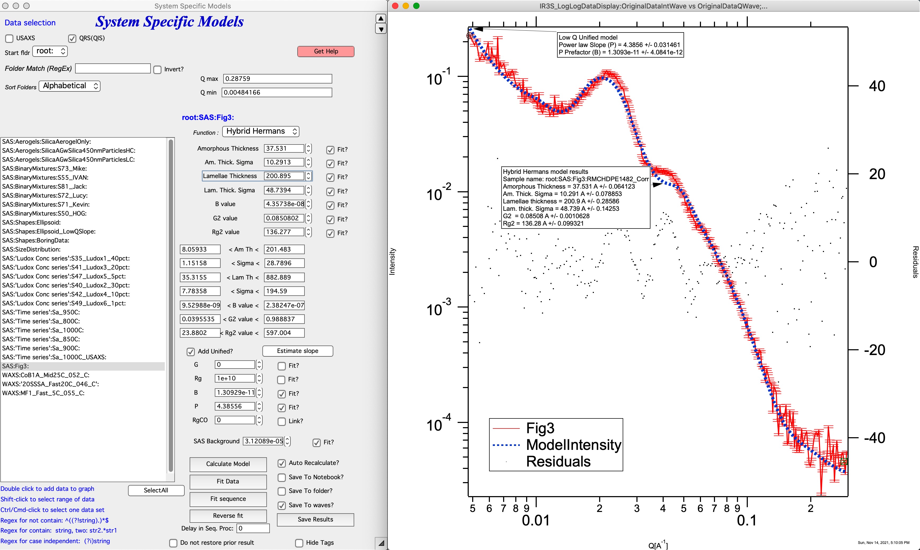
Note: this model has many parameters and solution uniqueness may be limited.
Unified Born-Green model for lamellar systems
Assumes laterally symmetric lamellae with a platelet structure and contrast only between amorphous and crystalline regions. Includes two-dimensional correlations between lamellar stacks (both thickness and lateral directions), unlike Hermans and Modified Hermans. Six parameters: Rg1, B1, p, ξ, δ, kI. Can be extended with additional parameters for higher-order structures.
For details: https://doi.org/10.1016/j.polymer.2021.124281
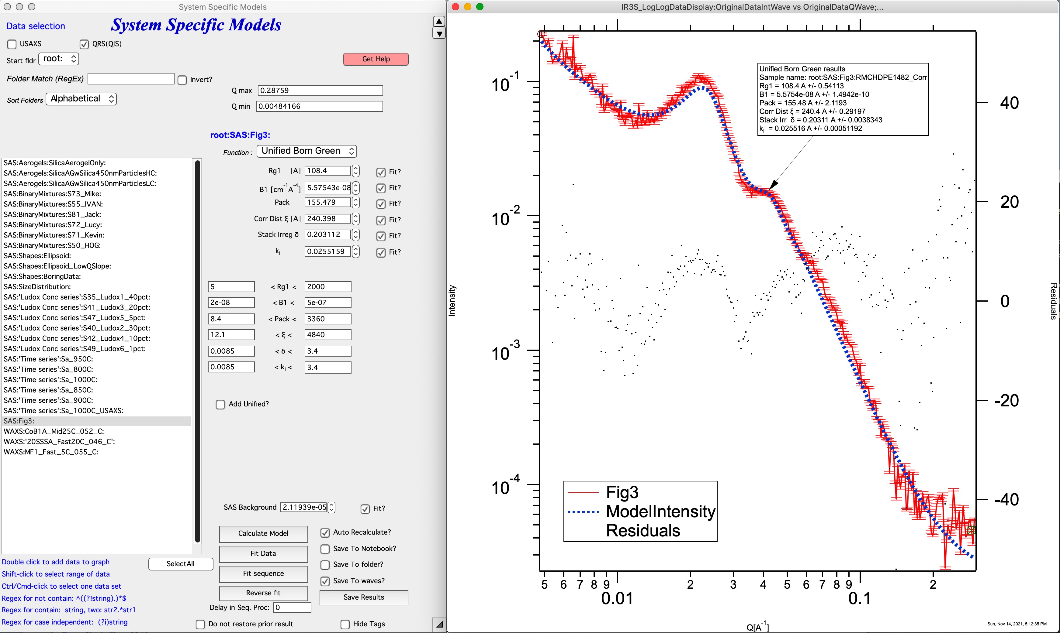
Note: this model has many parameters and solution uniqueness may be limited.